Introduction:
As part of a joint research project between the Gulf Fisheries Centre
(DFO, Moncton) and the Ocean Mapping
Group (UNB, Fredericton) an acoustic
survey was conducted of Shippagan Bay during July and August
2003. From it's southern tip to it's northern opening Shippagan
Bay is
approximately 15 km long. Shippagan Bay opens into the Bay of
Chaleur where the main
exchange of water takes place. There is an additional smaller exchange
of water between Shippagan Gully to the South and the Gulf of Saint
Lawrence.
The results of the above survey have two uses in this numerical
study. First, the bathymetry acquired from the survey
was used to generate a grid for the model. Second, the eventual
goal is to run the model for the same time as the survey so that we can
make a direct comparison between the model results and the survey
data.
|
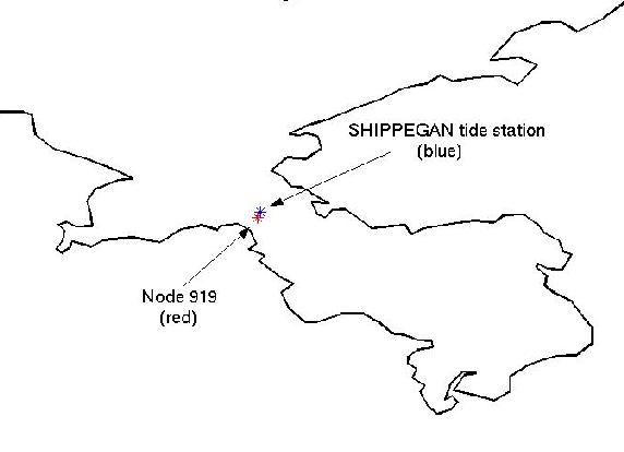
INSERT
MAP OF SHIPPAGAN BAY HERE
|
The
Numerical
Model:
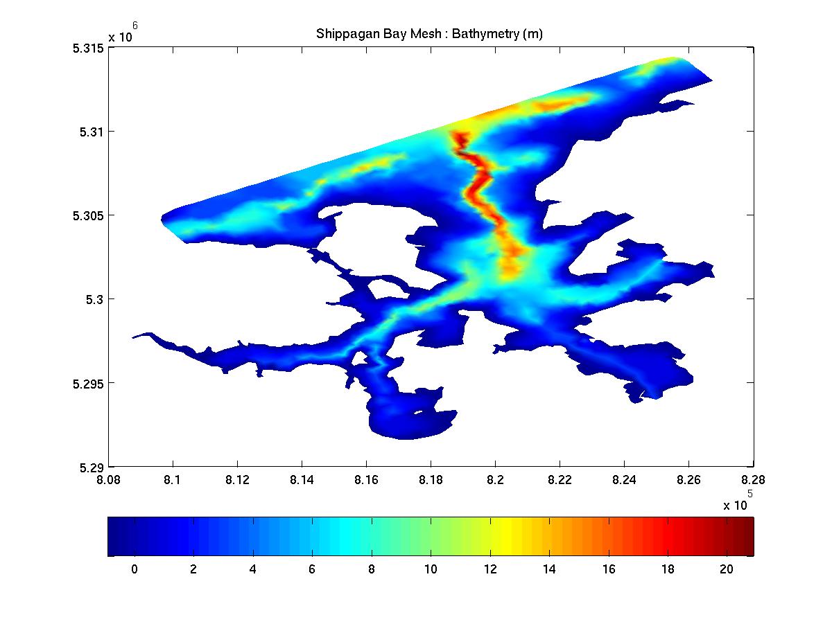
Shippagan Bay is
fairly shallow with a mean depth of approximately 4m. The bar
graph to
the right shows that most of the depth are in the [-0.9,10m] range with
negative values indicating above mean sea level. Because there
are
areas in the bay which are wet at high tide and dry at low tide, a
model that will allow for this is required. We are using the
finite element model Qu_dry which was developed by David Greenberg at the
Bedford Institute of Oceanography. Qu_dry is based on the
three-dimensional finite element shelf circulation model
QUODDY4_1.1A. In addition to the features of QUODDY which is a
non-linear, free surface, tide resolving model, Qu_dry allows for the
flooding and drying of intertidal areas.
|
|
Finite
Element Grid:
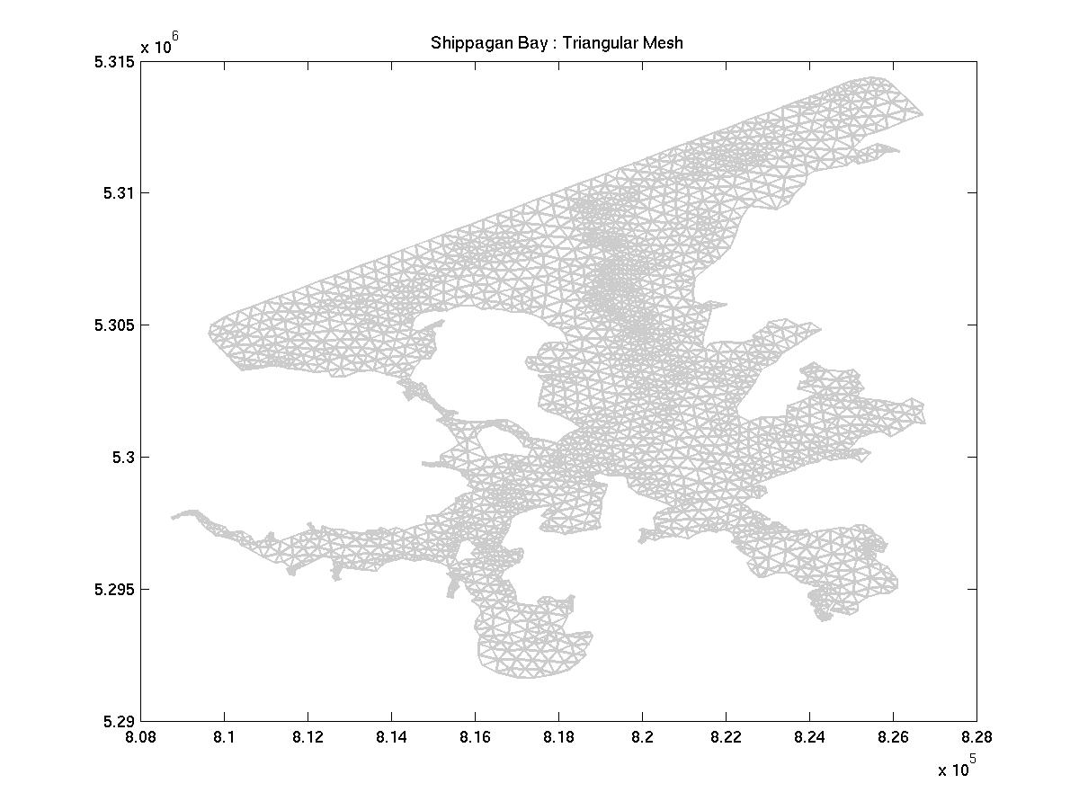
In order to
create a
finite element mesh, bathymetric data from the 2003 survey of Shippagan
Bay was used. The high and low tide water lines were manually
digitized from the Canadian Hydrographic Services Chart LC 4913.
A grid has been created which contains 2527 nodes and 4352
elements.
The depth range of the nodes is from -0.9m to 20.87m. The
elements
range in size from 1.2237e3m2to 1.0792e5m2.
At this time, we have 10 nodes in the vertical with a sinusoidal
spacing. |
Shippagan Bay Mesh
|
Shippagan
Bay Mesh: Bathymetry (m)
|
|