Squamish Lobe Deposits

The record of the June 14th 2019 "biggie" flow.
(and the largest in 2018 and 2017)
and 15 years of Squamish Distal Lobe Deposition

JEHC , CCOM/UNH
rushed draft to get things going ...
- September 2019

Hi Juan,

The figures and links below are a quick way to :

A - provide a surface and flow constraints for your modelling.
B - provide a quick update on the material I'm hoping to present at the AGU

Map Sheet Layout:

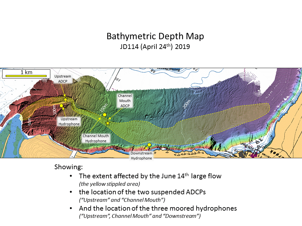
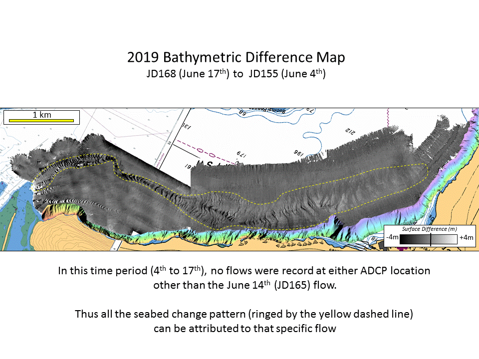
For almost all of the figures below, a common rotated map sheet has been used, aligned along the main axis of the Squamish channel-lobe system. That map sheet is illustrated in the figure to the right. It extends 7.4 km from the delta lip to the distal limit beyond which we currently can't recognize seabed change. For all figures below, the map sheet has been rotated anticlockwise by 123.2 degrees so that the flow enters from the left.

Notice that this is a significantly larger area than previously examined. During the early years (2011-2015), almost all the focus was on the proximal channels (see polygon in figure to right). And the last time the data were presented to Exxon (in 2017), the focus was on the growth of the South Channel (inset box in figure to right).

To help you in testing your models, you've requested observation for an example flow that we have measured (both flow characteristics and spatial extent of deposits) that extends from the channeled section, out onto the lobe. Below I am providing the preliminary information that we have on the largest flow record this (2019) year. Additionally, I'm providing preliminary information of two comparable flows for the previous two years.

The June 14th 2019 flow and deposits:

As an overview, the figures below shows you the area resolvably impacted by the singular June 14th flow this year. As you can see it was a single flow that had the longest runout we've ever recorded (see record of last 15 years at end of this report). Most significantly, although it was confined within the south channel for the first 4 km, it ran out onto the lobe for at least another 5 km.


If you want to see where on the planet we are click on this: http://omg.unb.ca/Projects/KML/Ortho_active_extent.EM710.JD11X_2019.kml

For your modelling purposes, you were asking for a DTM. I am providing that rotated map sheet that I use as a standard for all these figures. The grid is provided at 2m resolution and the pixel dimensions are:

3700 X
1100 Y

This grid is the channel and lobe as it as in April of this year - as each flow passes, the relief subtly changes. But this should be adequate for modeling the 2019 (and 18) flows. For each survey epoch, I have this same grid in the same format. All the surface difference maps that you see are just one array subtracted from the other.

The links below provide the grid bathymetry:

ASCII file (.llz) (97 Mb) containing lat-lon-depth values for all filled nodes
ASCII file (.asc) (39 Mb) containing a 2D array (size 3700x1100) matrix of depths (unfilled cells contain : -99999.000).

The upstream ADCP location is at:

49.672644 N -123.189593 W
in pixel coordinates of the provided array : 802 376

The Channel Mouth ADCP is at :

49.673450 N -123.207028 W
in pixel coordinates of the provided array : 1335 704

For interest, the three hydrophones were laid at:

49.674093 -123.1892 proximal_south
49.672317 -123.204155 mouth_south
49.672946 -123.222370 distal_south

I haven't processed those yet, but hopefully, all three heard this flow.

What we know about the June 14th flow:

As always it is hard to look inside these flows, particularly the ones that have such high concentration levels that attenuate the sound before its gets into the lower layers.

For the 3 week period of intense observations this summer we had two ADCPs in place (see location in figures and coordinates above). Nothing happened for the first 2 weeks before this flow.

For the upstream ADCP, we got a nice ~ 20 minute long record of the flow (see figure to left below).

For the downstream ADCP we only saw the first 50 seconds of it as it literally sucked the instrument down and into the flow, burying the instrument with the surface buoy dragged 110m underwater.

The record from the 1200 kHz ADCP at the upstream mooring

The record from the 600 kHz ADCP at the downstream mooring

The left hand plot is easy to interpret as the instrument remained 16m above the seabed and thus was unaffected by the flow. But the right hand plot is harder to comprehend and thus needs some explanation:

The bottom profile on the right hand plot shows the depth of the instrument and from that one can see that, at the moment the flow hit, the instrument package was dragged down to the seabed within about 50 seconds. After that time, the data is meaningless as the instrument is on its side being dragged along by the flow.

Fortunately, in 2019, we increased out logging interval from 20 seconds to 0.8 seconds so that we got over 60 samples of the flow before losing the data. By comparison, in 2017 when (in hindsight) we now realize that the same thing happened, we were using only 20 second sampling (due to memory and power constraints) and thus we only got ~2 (corrupted) samples before the instrument hit the seabed.

At this time I haven't done more than look at the flows with WinADCP (figures above). So for now I think you could start your model with some simple dimensions:

Upsteam Flow:

head thickness of 8 m
head speed of 3 m/s
body thickness of 10-12m
sustained body speed of ~1.5m/s for 15 minutes.

Downstream Flow:

head thickness of 5 m
head speed of 5 m/s
body thickness unknown
body speed of ~2.5m/s for an unknown period.

Average Speed between Moorings:

Note that for both these flows, it is clear that the acoustic pulse were not able to penetrate through the head of the flow and thus the velocity estimates are probably lower than reality as we are just sampling the more dilute upper parts of the flow.

We can however, use the transit time from the upstream to the downstream mooring to estimate the average speed of the head between the two points. It traveled about 1300m is 285 seconds - thus:

averaging : 4.6m/s

Note that this is a LOT faster than the apparent body speeds.

Hydrophone Recordings:

We do also have the potential to get more information about the flow from the hydrophones that we had recording throughout event (see locations in figure above). We haven't yet analyzed this data though. There was one hydrophone adjacent to each of the ADCPs. so we can calibrate it using the upstream flow, for which we have a complete record. We can then hopefully get a better view of the duration of the flow at the Channel mouth (the point at which it was sucked down).

But most interestingly, we added a third hydrophone on a terrace downstream on the lobe. I am hoping... that this will provide a third constrain (arrival time, duration and possible indicator of speed).

Other flows :

Originally I thought that just this (2019) year's data would be suitable for your modelling, but, going back over the 2017 and 2018 data I now think there are two other singular flows that you may be able to use also. I'm proving brief information at this point in time:

The June 2018 flow and deposits:

In 2018, we had just the Channel Mouth ADCP in place, but during a 2 week window, there was one significant flow which resulted is a rather similar morphological signature on the lobe (see left figure below).

The big difference in 2018 (and 2017), is that with less memory and batteries, we were only storing the ensemble average of the currents every 20 seconds and thus much of the detail we now see in the 2019 data (every ~ 1 second) is averaged out.

For the 2018 flow, what was remarkable was that, for a single 20 second epoch the average velocity at the bottom of the flow was 10m/s Given that this is a single observations and the average for the preceding and following ensemble is much smaller, I'm not sure I believe it. This is why we now have hydrophones and pressure triggers along the lobe, so that we can get transit times.

I'm not sure what #'s you might use from the figure to the right. Perhaps a surge with a peak > 5m/s for about 2-3 minutes followed by a waning body that drops to 1m/s after about 20 minutes. As to thicknesses - the head and the bosy almost reach the instrument (14m of the channel floor).

The June 2017 flow and deposits:

In 2017, we had the same single ADCP suspended above the channel mouth. While we recorded many flows, there were only two that were fast enough that they probably made it out onto the lobe. At the time, I focused mainly on the one with a peak 6.5 m/s head. But we also had a second event which we didn't understand at the time. The instrument abruptly (within two 20 second ensemble averaging periods) dropped to the channel floor and thereafter the data was rubbish. In hindsight, it probably did exactly what we saw this year, with the instrument being sucked down by the flow.

The figure to the left below shows the seabed change associated with one or both of these flows and the figure to the right shows the flow we managed to record.

The seabed change recorded over a 33 day period in which only two significant flows occurred.	The record of the first of those two significant flows.
The record of the second flow ( we think) in which the instrument abrupt drops to the channel floor.

The Full record of the Distal Lobe Deposition over the past 15 years:

For the three periods in the last three years, illustrated above, one can see that occasionally (about 2-4 x per year) flows coming down the south channel are of sufficient magnitude that they escape the channel, pass through the CLTZ and spread out on the lobe. Of course, this is dependent on the location of the channel mouth. Since 2004, we have been surveying this area, and have watched that channel grow. Most notably, in 2017, I presented to you the evidence of its rapid extension in the 2009-2015 period. After that, I've been waiting patiently for the channel to grow some more. I think, in the last 2 years (the period during which the three flows illustrated above occurred) we have started to see a new section of the channel develop on the proximal lobe.

This is the story I'm hoping we can present at the AGU. To jump-start discussions, I've provided all the surface differences we have compiled over the past 15 years of flows that have extended out this far (all using that same rotated map sheet aligned along the system with the flows entering from the left):

A - 2004 and 2005 seasons

This was the first ever pair of surveys. This was long before the South Channel extension formed. The upper South Channel was actively entrenching. The distal lobe seemed to get as much sediment from the North as the South Channel. Bedforms distally are all simple long wavelength forms that are laterally extensive.

Note that, with these early surveys, there are lots of bathymetric artifacts due to imperfectly calibrated systems, thus much of the background grey level fluctuations that you see are not real. I hope you can see past this to recognize the periodic signature of the migrating dunes.

B - 2006, 2007 and 2008 seasons
While there were surveys of the shallower section (< 150m) within this 3 year time frame, none of them extended out onto the lobe. The 2005 and 2009 surveys are used to see the cumulative change out on the proximal lobe. Compared to the previous 2 years, what is remarkable is how little the flows extended. One reason might be that the upper South Channel was acting as a storage reservoir and containing most of the off-delta flux.

C - 2009 and 2010 seasons

In the following 2 years, the situation changed remarkably. The South Channel extension first formed in this period, cutting its way through and down into the old proximal lobe. Again, both South Channel and the North Channel appear to be responsible for the movement of long wavelength, laterally extensive bedforms on the more distal lobe.

D - The 2011 Summer

This was the summer in which we did 5 months of daily surveys. On the basis of this data set, much of the recent publications are based. There were indeed over 100 flows recorded. Yet not a single one in that summer made it out onto the distal lobe. Thus none of what we've been describing had any influence on the distal lobe.

E - 2011-2012 Winter

Over the following winter (and half way through the following summer), movement of those long wavelength bedforms on the lobe restarted. In this period, the South Channel extension actually back filled a bit.

F - 2012 Summer and 2012-2013 Winter

In this period the South Channel extension flushed out and the most extensive and distal evidence so far of lobe bedform activity appeared. The influence of the North (and Central) Channels appears to wane from this point onwards.

G - 2013 and 2014 seasons
The South Channel extension stabilized during this period so that, at the start, flows were spilling overbank quite a bit upstream, but this increasingly stopped with time. On the proximal lobe downstream of the current channel mouth, there is net accretion and pretty simple long wavelength bedforms that extend across the lobe.

H - 2015 Summer and 2015-2016 Winter
Finally the South Channel entrenchment has got to the point that there is no overbank spillage until we get to the ADCP location. during this 12 month period, the first indicator of nucleation of that proto-channel on the proximal lobe started.

I - 2016 Summer
growth of that proto-channel. Just long wavelength broad low bedforms downstream of that.

J - 2016-2017 Winter
Remarkable distal extent of activity. Note that, beyond the nucleation point, the bedforms are long wavelength and broad, suggesting there is not a specific talweg to follow.

K - 2017 Summer
The south channel mouth has been a depo-centre and thus has shoaled, encouraging the flows to leave the channel earlier and spread out. Better definition of the corridor upstream and downstream of the nucleation point. There appears to be a "bypass zone" between the proximal lobe and the distal lobe in which there is strangely no record of any bedform activity (or erosion or deposition) at all?. This is the point at which the flows are forced to turn slightly to the left due to the presence of the fjord wall.

L - 2017-2018 Winter
Despite low discharges, plenty of distal lobe activity. First definition of shorter wavelength bedforms along an apparent preferred downstream talweg.

M - 2018 Summer
increasing definition of the shorter wavelength bedforms in the developing downstream talweg.

N - 2018-2019 Winter
An unusually quiet winter. But there was one (or more) flows that made it out onto the lobe. But, these were not sheet flow events. Rather they only followed along the gradually developing shallow talweg, just moving those shorter wavelength bedforms.

O - 2019 Summer
This is the change observed this summer (so far) from April to end of June. It includes the singular huge flow on June 14th. Prior to that, the April to early June survey differences confirm that nothing exited the South Channel.
Note the discharge for the rest of the summer until now (July to September). This has been a particularly anomalous wet summer in BC with unusually sustained discharge and two notable major surges. Three pressure gauges are deployed in line along the distal lobe so, hopefully next week, we we will see both A : - whether any more big flows happened and B: when they occurred.

All for now ....

Heading to Squamish tomorrow for the last surveys of the year (and then put the Heron to bed for the winter). I will compile a more complete report in November once all the data is in.

Cheers John

page created by JEHC, Autumn 2019