Results:
We are
running
QUODDY in the baroclinic mode. The model
starts at rest
with zero elevation everywhere. The elevation and normal
velocities are slowly ramped up
over the first tidal cycle. We run the model for a total of six
tidal cycles and examine the results. There are two areas in
which we are interested : the Saint John River portion of the model and
the entrance to Kennebecasis Bay.
First we examine the Saint John River portion of the model. The
dynamics of the Saint
John River are controlled by the forcing at
the open boundaries Brandy and Gorge. Thus it is important
to know how well the model reproduces the boundary conditions at the
two open boundaries. As we are relaxing towards temperature,
salinity and normal velocity at the boundary, we expect the model to
reproduce the measured values reasonably well. Figures 6 and 7
show the modelled elevation, temperature, salinity and normal velocity
at the Brandy and Gorge boundaries respectively. Comparing these
with the measures values in Figures 3 and 4 we notice that the model
predicts reasonable temperature and salinity structures when water is
flowing into the domain which occurs during the ebb tide at Brandy and
the flood tide at Gorge. It is of interest to note that at
both Brandy and Gorge, the bottom salty water in the model is less
salty than those observed. There are also differences in
temperatures. When water is flowing out of the
model
boundary during the flood tide at Brandy and the ebb tide at Gorge,
temperature and salinity structures are more influenced by the modelled
temperature and salinity inside the model domain and do not match the
observed values as well. In particular, the lower salty layer at
Gorge almost dissappears during the ebb tide.
Normal velocities are reproduced reasonable well in terms of direction
and timing throughout the tidal cycle. At Gorge, the amplitudes
of the velocity are less at all phases of tidal cycle. At Brandy,
the upstream flow during the flood tide is stronger in the model than
observed.
|
Figure 6:
Modelled elevation, temperature, salinity and normal velocity at the
Brandy
boundary. Results are for node 4060 in the center of the
Brandy boundary (see Figure for location).
|
Figure 7:
Modelled elevation, temperature, salinity and normal velocity at the
Gorge boundary. Results are for node 5014 in the center of the
Gorge boundary (see Figure for location).
|
The
differences in the modelled and observed temperature and salinity
mentioned above lead us to question how well the model conserves the
total
salt and heat. Ideally, over a tidal cycle, the total heat/salt
flux
at Brandy would equal the total heat/salt flux at Gorge.
Approximate
total heat and salt flux at the
Brandy and Gorge boundaries are computed for the last four tidal cycles
of our simulation and are given in Table 1. These flux are
calculated
by integrating the heat/salt flux, T/S*vn, over the
cross-sectional area of the boundary and then integrating this over an
entire tidal cycle. The normal velocity, vn,
is defined as being positive downstream. Thus a positive/negative
flux
at Brandy means that there is a net gain/loss of heat/salt. A
positive/negative flux at Gorge means that there is a net loss/gain of
heat/salt. The values in Table 1 show that both fluxes at Brandy
and Gorge are contributing to a net decline in temperature and salinity
of our model domain.
|
Tidal Cycle
|
Total T Flux
Brandy
|
Total T Flux
Gorge
|
Total S Flux
Brandy
|
Total S Flux
Gorge
|
3
|
-2.3e7
|
1.5e8
|
-4.0e6
|
6.8e6
|
4
|
-2.1e7
|
1.5e8
|
-3.9e6
|
6.9e6
|
5
|
-1.9e7
|
1.6e8
|
-3.8e6
|
7.1e6
|
6
|
-2.2e7
|
1.6e8
|
-4.0e6
|
7.0e6
|
Table 1:
Next we examine how the
model behaves in the interior of the model domain. We know that
there is
residual
downstream flow from Brandy to Gorge. We expect the model to
reproduce
this residual flow as the elevations used to force the boundaries have
residuals of 4.8cm at Brandy and 0cm at Gorge. Figures 8 and 9
show the M2 residual elevation and the vertically averaged residual
velocity fields. These show a decrease in the elevation
from
Brandy to Gorge and a net downstream flow.
|
|
Figure 8: M2 residual fields
|
The flow in the Saint John
River portion of the model is a balance between the river's fresh water
discharge and the salt water brought in from the Bay of Fundy by the
tides. Although there is a net downstream flow due to the
river's discharge into the Bay of Fundy, the tide affects the direction
of the instantaneous flow as well as the water properties. It is
useful to explain the flow in terms of the actions of the tide at
Gorge. During the flood tide, cold salty water from the Reversing
Falls enters the Saint John River at Gorge. This pushes the water
upstream causing a reversal in the rivers flow. As high tide
approaches, the river 's velocity slows downs and then does an about
turnjust after high tide. Figures 6 and 7 indicate that the
normal velocity at Gorge reverses before that at Brandy indicating
that, as the tide receeds, water is being sucked out of the Saint
John River into the Bay of Funday. At low tide, the flow
is dominated by the
river's fresh water discharge. At Brandy, there is a permant two
layer density structure with fresh warm water lying over cool salty
water. To illustrate how the model is performing in the
Saint John River, we have chosen to examine a transect from Brandy to
Gorge. Figure 10 shows the instantaneuos behaviour of the model
along a transect from Brandy to Gorge during the flood tide just before
high tide. At this point, the water is
flowing upstream and cold salty water
from the Reversing Falls is still entering the Saint John River system
at Gorge. We observe that the cool salty water flowing upstream
from Gorge doesn't protrude far enough upstream to join with the cool
salty water on the Brandy side. In fact these two water segments
always remain detached. At first we thought that this was a
problem with the model but observations made on JOHN DATE AND PICTURE PLEASE and
shown in Figure 11 show that this is indeed what happens. This
indicates that the cold salty water at Brandy does not get renewed each
tidal cycle but depends on the strength of the tides and the river
runoff.
|
Figure 10:
Instantaneous flow along a transect in the Saint John River
from Brandy to Gorge. The transect is indicated by the black line
in the vertically averaged velocity field figure. For plots of
temperature, saliity, and tangential velocity, Brandy is located at the
left end and Gorge at the right. The * on the Brandy boundary is
node 4060 and the *
on the Gorge boundary is node 5014.
|
*************JOHN FIGURE
PLEASE*************
Figure 11:
|
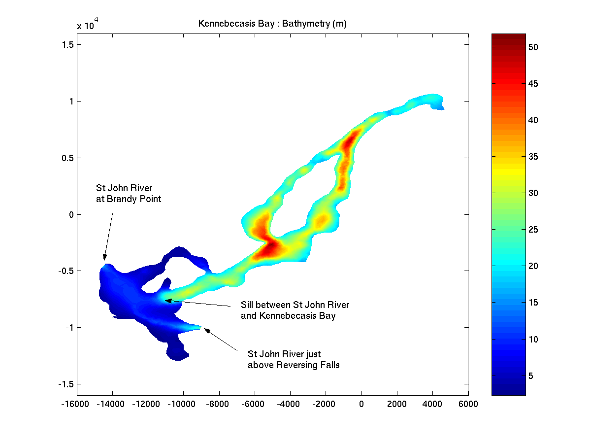
Finally we examine the
flow from the Saint John River into Kennebecasis Bay.
Kennebecasis Bay is a fjord-like estuary. It is deep (up to 60m
deep in spots) and has a permanent pycnocline with warm fresh water
lying over cold salty water. The water in Kennebecasis Bay has
very little movement although we know from Trites (1960) and from the
13 June 2003 survey that water can be injected into Kennebecasis Bay
from the Saint John River at high tide. Figure 12 shows the
instantaneous flow in Kennebecasis Bay along a transect from the Saint
John River into the bay. The flow is shown at the
beginning of the ebb tide when the water in the Saint John River is
flowing downstream. This corresponds to the same phase of the
tidal cycle shown in Figure 5. Comparing figures 5 and 12 the
first thing that we notice is that the observed temperature and
salinity is cooler and saltier than the modelled temperature and
salinity. NEED TO TIE THIS
IN TO SALT AND HEAT BUDGET. Anotherdifference worth noting is
that the modelled pycnocline is significantly thicker than the measured
pycnocline. This is likely due to the diffusion coefficient used
by the numerical model being larger than the actual physical diffusion
in Kennebecasis Bay. As there is little water movement in
Kennebecasis Bay, the vertical mixing of temperature and salinity is
determined by the diffusitiy of these agents. In pure water the
diffusivity of heat and salt (.01 molar) at 15°C is 14x10-8m2/s
(Fischer et al., 1979) and 0.1493x10⁻⁸m2/s (CRC
Handbook of Chemistry and Physis), respectively. In QUODDY, we
set the minimum vertical eddy diffusivity for heat and salt to 10-4m2/s.
This larger diffusivity value is required for numerical stability
(CHECK THIS) but has the dissadvantage of predicting more vertical
diffusion than is actually present. In areas where the flow is
dominated by the tide, this effect is not as noticeable.
One feature of the numerical model is that it predicts a
flow in Kennebecasis Bay itself. Figure 12 shows that there is a
flow into Kennebecasis Bay in the surface waters and a return flow in
the bottom waters. We know that this flow is a numerical
artifact. After some investigation we believe that this flow is
due to an error in the calculation of the baroclinic pressure gradient
in sigma coordinates when there is a sudden change in topography.
|
Figure 12:
Instantaneous flow along a transect from the Saint John River into
Kennebecasis Bay. The transect is indicated by the black line
in the vertically averaged velocity field figure and follows the
transect of the 13 June 2003 survey (see Figure 5). For plots of
temperature, saliity, and tangential velocity, the Saint John
River is located at the
left end and Kennebecasis Bay at the right. The *, *, and * in the vertically averaged
velocity field indicate the locations at which the elevation is shown.
|
|