MUSQUASH ESTUARY: NUMERICAL MODEL

The Model:

The Musquash Estuary is a macrotidal coastal estuary.  It is subject to tides from the Bay of Fundy which are known to be amoung the largest in the world.    The Musquash Estuary has an average tidal range of 6m.  A result of the high tides is that the volume of water in the estuary at high tide
(7.45x10⁷m3)  is roughly six times that at low tide (1.23x10⁷m3).   The Musquash Estuary has large areas of mudflats which, although covered by  water at high tide, are exposed at low tide.   In order to properly model the Musquash Estuary, a numerical model that allows areas to be dry at low tide and wet at high tide is required.  We are using the finite element model Qu_dry which was developed by David Greenberg at the Bedford Institute of Oceanography.  Qu_dry is based on the three-dimensional finite element shelf circulation model QUODDY4_1.1A (Lynch et al, 1996).  In addition to the features of QUODDY which is a non-linear, free surface, tide resolving model, Qu_dry allows for the flooding and drying of intertidal areas.


Finite Element Grid:

A triangular grid was generated using BatTri (Biligili et al. 2004), a Matlab interface to the finite element grid generator Triangle and then refined using the grid generation program Genesis (developed by Florent Lyard).  Bathymetry was obtained from three sources.  In September 2001 the Ocean Mapping Group (OMG) conducted a survey of the Musquash Estuary.  Although extremely dense, the coverage obtained from this survey does not include the entire area of the estuary. Additional bathymetric depths were obtained from the Canadian Hydrographic Services (CHS) chart of the area: LC-4116.   As our model domain extends into the Bay of Fundy, we use depths from the 15 second resolution digitial bathymetry of the Gulf of Main created by E. Roworth and R.P. Signell (http://pubs.usgs.gov/of/of98-801/index.htm) for areas not covered by the other two data sets.  The high water mark was manually digitized from an aerial photograph of the estuary and used as the model's coastline.  The coverage of the bathymetric data used is shown below to the left.


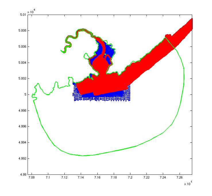
Areas shown in red are from OMG's multibeam data, those in blue are the CHS chart data.  The grid's boundary is shown in green


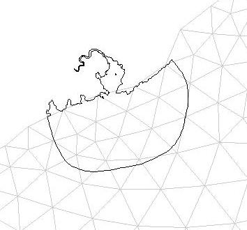
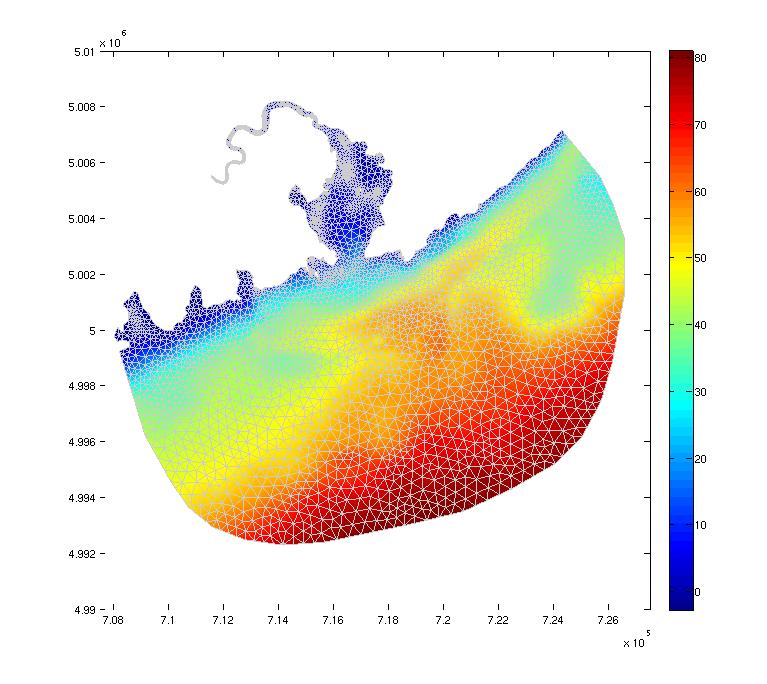
Finite element grid: 4174 nodes, 7618 triangular elements, and 732 boundary nodes.

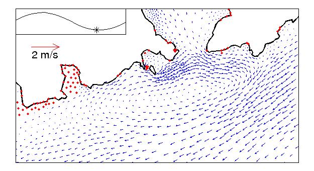
In September 2001, the Ocean Mapping Group conducted an ADCP study of the Musquash Estuary.  The purpose of this study was to better define the seaward boundary of the then proposed Musquash Marine Protected Area.  Results from this study were used to help us decide the extent of our model domain and where to densify the nodes.   In particular we chose to densify the grid to the South of Gooseberry Island extending to Western Head and to the South of Musquash Head.

The resulting mesh is shown above to the right.   There are 4174 nodes and 7618 elements.  The elements range in size from 234m2 to 124910m2.  The depth ranges from -2.8m to 81.0m where a negative depth indicates a depth above mean sea level.

Boundary Conditions:

The finite element mesh of the Musquash Estuary has an open boundary to the South which extends roughly 10km into the Bay of Fundy.  Boundary conditions for this open boundary were obtained from WebTide.  The underlying data files contain  the M2 constituent of the elevation in the Bay of Fundy.  The values along our boundary were interpolated from the WebTide values closest to our boundary.  The data used has a tidal amplitude of approximately 2.9m giving a tidal range at the open boundaries of 5.8m.  The model is started from rest with zero elevation everywhere.  The elevation on the boundaries is ramped up to the forcing values over the first tidal cycle.  The model is run for a total of 12 tidal cycles.  Results are shown for the last tidal cycle.


Musquash grid boundary embedded in WebTide grid

Results:

We run the model in the barotropic mode implying that our estuary is well mixed and has little variation in temperature and salinity.  This is a reasonable approximation for circulation of the lower estuary but ignores density variations from two sources:  the minor Musquash Watershed discharge and the influence of the Saint John plume.  The only forcing is at the open boundaries where the elevation is imposed at the above mentioned values. 

Below is the M2 residual velocity field.  There are several features worth noticing.  Firstly, water tends to enter the estuary along the western shore and exit on the eastern shore.

    
Residual current: click on image to see enlargement of area bordered by green box.

The following 12 images show sequential stages of the tide at roughly hourly intervals.

FLOOD TIDE
EBB TIDE


Animation files:

Right click here to download animation of current field for central estuary and upper saltmarsh area.
Right click here to download animation of current field for estuary mouth and offshore.

Compare to observed currents at : ADCP_experiment