Using Webtide for OMG processing

Running tidecor2.42
You can run this program in one of four ways:

1. -onto_nav, pass a .nav format input and output file. The input file must contain position and time, the output will contain the same with the water level stuffed into the 'azimuth' field of the record (can modify to shove into depth or velocity field with command line switches -into_depth and -into_vel, respectively).
2. -onto_merged, pass a .merged file as the input file.
3. -onto_grid, pass an OMG .r4 grid as the input file. Tidal amplitude (or phase) values will be calculated for each grid node based on the chosen constituents (through the use of -amp or -phase switches, respectively). You can choose which constituent with -M2, -S2, -N2, -K1 or -O1.
4. -get_coeffs_at, pass a latitude and longitude and select a model. Will print out constituents for the provided position.

1. Automatic: Syntax is -model_map MODEL_MAP_NAME, e.g. -model_map $ARCTICNET_MAPS/tidecor_models.8bit. Alternately, you can specify any model map you like. Check out the notes on creating model selection maps below for more details on how to create this kind of map. The format is an OMG 8-bit georeferenced mapsheet with areas for each model encoded using the following codes (COMPLETELY arbitrary encoding):
   • 11 halifax_harbour
   • 12 hudson_bay
   • 13 northwest_atlantic
   • 14 arctic
   • 15 northeast_pacific
   • 16 scotian_shelf
   • 17 upper_fundy
   
   

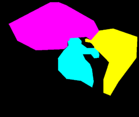
   An example of such a mapsheet is shown on the right, in this case, the Arctic model is magenta, the Northwest Atlantic model coverage area is yellow. Cyan is the area covered by the Hudson Bay model. Note that this map represents areas in which a model will be forced, even though the requested point may lie in another model as well (e.g. overlap between Arctic and NW Atlantic models in southern Baffin Bay).

2. Manual: Syntax is -model MODELNAME. You specify the MODELNAME from the following list:
   • Arctic
   • Halifax Harbour
   • Hudson Bay
   • Northeast Pacific
   • Northwest Atlantic
   • Scotian Shelf (includes Bay of Fundy)
   • Upper Fundy
   The model name provided on the command line must match the corresponding model subdirectory in the TIDECOR_PATH directory (see notes about environment configuration below). More details about the spatial extent of each model can be found on the Webtide website.

Optional arguments:
-time_shift N: You can add a time shift of N minutes with the -time_shift option, the shift is additive, i.e. it is added to time values prior to tide calculation.
-use_nearest: You can force the usage of the nearest node value when the locations in the input file wander off the mesh. The default is to give a water level of zero at these locations.

The following example shows how to apply tides to a .merged file with a time shift of 60 minutes (60 minutes is added to the record time).

    tidecor2.42 -model arctic -onto_merged -in 0045_20060728_161954.merged -time_shift 60

Known Issues

• When your input file wanders outside the model bounds, a tide of '0.0' is applied. Seeing as MSL is the vertical datum, this could be confused with an actual water level of zero, so we should decide on an appropriate 'no data' value for the tide field in the OMG profile structure. Having done that, the program should be modified to use this value for areas outside of the mesh.

Additional Notes

    setenv TIDECOR_PATH /homes/share/datasets/WEBTIDE

Config File Format
The configuration file (always named tidecor2.4.cfg) contains the filename of the .nod and .ele files for the model of interest. The next value is the number of constituents included in the model. The list following the number of constituent values consists of constituent name and filename associated with the constituent.

arctic8cll.nod
arctic8c.ele
5
M2
M2.barotropic.s2c
S2
S2.barotropic.s2c
N2
N2.barotropic.s2c
K1
K1.barotropic.s2c
O1
O1.barotropic.s2c

Adding new models
If you have a new modelled area to add (e.g. Sue's Musquash model), do the following:

1. Add a subdirectory for your model in the TIDECOR_PATH
2. Copy the model output files into the new subdirectory.
3. Create a configuration file in the subdirectory that obeys the file format discussed above.

Creating model selection maps

# Create yourself a mapsheet of the model coverage using the -onto_grid feature of tidecor.
# This mapsheet will provide you with a backdrop against which you will manually define the 
# outermost bounds.  Make sure that your initial basemap (1) covers your area of interest,
# and (2) is of a sufficient resolution to adequately model the boundary of the model domain
# in the area that you're working.
tidecor2.42 -onto_grid -amp -M2 -in model.r4 -model arctic

# Now create a .8bit file.
r4to8bit model

# Now jview the .8bit file with the -mask option.  Middle click in the map window to create nodes 
# of a polygon that covers the area that you want to force the usage of this model within.
# You can use the 'u' key to undo and remove bad points.  The program will automatically close
# the polygon for you so there is no need to click the start point a second time.
# Once you're done, make sure you click the 'EXIT' button to exit jview cleanly.
# It will write out a file named mask.file which will contain the polygon coordinates
#  (in pixel space within the mapsheet).  
jview model.8bit -mask

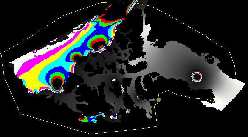
An example of making a mask is shown in the image below (click for high-res). The M2 amplitudes are mapped out for the Arctic model. The yellow line is the user-selected area of the mask. Note that the mask was deliberately chosen to clip off use of the Arctic model in areas of overlap with the Hudson Bay model (Fury and Hecla Strait) and the Northwest Atlantic model (Davis Strait).

# This step takes the mask.file coordinates and generates a mapsheet with the polygon painted
# in with the value specified by -val.  The value specified must match the code names listed
# earlier, e.g. the arctic model has a code of 14.
mask_make -val 14 -infile mask.file -outfile arctic.mask

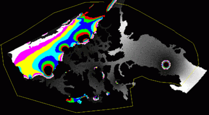
The above process would be repeated for all models of interest. An example of the Arctic mask map is shown below.

# Once you have all of your model mask files created (with the correct encoding), you can use 'add8bit' to collapse
# them into a single mapsheet.  You'll need one or more temporary files depending on how many models you need to 
# join.  The -max switch in add8bit forces the program to always preserve the maximum encoded value in case any of
# the models overlap.
add8bit -max -first arctic.mask -second hudson_bay.mask -out temp.8bit
add8bit -max -first temp.8bit -second northwest_atlantic.8bit -out model_selection_map.8bit

# Now we need to get an image header into the mask file.  Use the initial model map to provide an image header for us.
# This provides us with a fully geo-referenced model encoded mapsheet for use in tidecor.
edhead -replacehead model.8bit model_selection_map.8bit

Here are a few useful commands for having a look at what's actually inside the various model files.

# This will dump out current and tidal height values for the all the nodes in 
# any of the webtide model files.  Note that 'readQUODDY' expects the .nod and .ele
# file to have the same prefix so we must copy arctic8cll.nod to arctic8c.nod before we
# begin (since the .ele file has the name arctic8c.ele).
cp arctic8cll.nod arctic8c.nod
readQUODDY -model arctic8c -tide M2.barotropic.s2c -curr M2.barotropic.v2c -out temp

# This draws all of the triangular elements as a mesh on the underlying map
jview $ARCTICNET_MAPS/canada.sun -vector temp.ele_out

# This plots tidal vectors at all the node locations
jview $ARCTICNET_MAPS/canada.sun -tide temp.mocktide -currents -navlook temp*currvec

# There's quite a pile of temp files laying around, clean them up if you like.
rm temp*