CSL Heron 2018 Operations
Squamish Experiments
EM710/2040P - ADCP - DDS-9001 - Hydrophone -
Pressure Gauges
April 8th to October 17th, 2018
John E. Hughes Clarke
Liam Cahill
Brandon Maingot
|
Ian Church
|
Anand Hiroji
|
Carlos Vidiera Marques |
Center for Coastal and Ocean
Mapping
University of New Hampshire
|
Ocean Mapping Group
University of New Brunswick
|
Dept. Marine Science
University of Southern Mississippi
|
Hydrographic Institute
Portuguese Navy
|
Technical Support: Gordon Allison
(CCG retired) and Mike Boyd (Polar Diving)
Executive
Summary
Primary
Findings - Summer 2018 Field Season
The 2018 summer field season of the CSL Heron, extended from
April to October and involved deploying a variety of sensors across
the active part of the Squamish prodelta.
|
|
2018 instrument
deployments on morphology
|
2018 instrument
deployments on surface difference |
Whether for turbidity current research, seabed change detection or
sonar performance, the following most significant findings of the
2018 Squamish field season include:
- Demonstrating that high velocity (~>1m/s) Turbidity Current
Flow events have a distinct acoustic signature.
- That this signature can be separated from the background
noise, even though it has become apparent that there is a very
significant anthropogenic noise problem in upper Howe Sound.
- That, while multiple events are present (at least 20 as
detected through passive acoustics) only two events in the
entire period (April to October) extended significantly beyond
the mouth of the Southern Channel.
- The largest event of the year (the fastest ever actually
detected), peaked at 10 m/s (20 knots) as measured at the
ADCP location. It was responsible for the furthest extent
of resolvable seabed change and appears to have dragged two 100
lb mooring weights (PG3 and PG4 see figure above) over 200m at
the most distal extent.
- The DDS-9001 was successfully deployed and operated for
the first time from the CSL Heron
- Despite only being deployed to a depth of 40m (due to cable
limitations) the DDS-9001 clearly showed that it is capable of
imaging a circular area with a diameter of 1.5 km, with a
~ 2 second update.
- The pressure gauge moorings have proved their worth again.
While only one of the 4 gauges was recovered in October (due to
winch failure), they have all been periodically located using
acoustic tracking. It is apparent that two of the gauges have
been dragged over 200m down flow.
- The one gauge that was recovered in October (off the Northern
Channel) provided a complete 10 second interval record for the
full 7 months (in 2017, a hardware fault in the instrument
terminated the logging after only 21 days).
- After removal of the tidal signal, the timing of flow events
can be clearly discerned. Strangely, the Northern Channel
appears to have been most active only in August well after the
river has dropped?
- As well as a pressure signal related to vertical movement of
the gauge, in late September, there were distinct thermal events
that appear to be related to a river surge. It is speculated
that this is a record of an injection of warm water at depth
(presumably entrained by the turbidity current), that provided
an indicator for a flow, even if the gauge is not in the path of
the main flow.
- The scour depression on the proximal Southern Channel
lobe is slowly growing into a headless channel thereby
increasingly capturing the unconstrained flow.
- The proximal Southern Channel lobe is developing two possible
preferred pathways (one of which is the scour induced corridor).
- Both pathways, ultimately lead obliquely into the fjord wall.
It is apparent that the flow is then deflecting off the fjord
wall and forming a new even-more distal preferred pathway
extending out toward Woodfibre.
- At the most distal extent of resolvable change there are two
distinct styles of bedform activity :
1 - a broad corridor within which long wavelength bedforms
migrate (without significant scour).
2 - a narrower corridor following the lowest point within the
broader corridor, within which shorter wavelength bedforms are
developed that exhibit significant erosion.
Overview
and Experimental Intent
Scientific/Engineering Objectives
The 2018 Squamish operations are a continuation of a long-standing
experimental configuration that started in 2006 when the main author
was at the University of New Brunswick. Its year-to-year
continuation depends on maintaining funding (see below) and meeting
the specific objectives of all the partner organizations.
Deployment Timing
CSL Heron operations began in early April with mobilization from the
Institute of Ocean Sciences in Sidney BC and ended with a final
demob. at the same location in October. There were three
operational windows in between - end May, mid June and Late June.
Manning:
- April - Hughes Clarke and Marques
- May - Hughes Clarke and Boyd
- June A - Hiroji, Hughes Clarke and Cahill
- June B - Hughes Clarke and Boyd
- October - Hughes Clarke and Maingot
Gordon Allison of course, was there as skipper for all
deployments.
Mike Boyd, of Polar Diving was there for the May and June B
deployments to assist in the DDS-9001 logistics and ADCP deployment
and recovery.
Funding Agencies
The Squamish Operations are funded jointly by three agencies with
separate objectives which happen to share logistics in a common
location :
- Exxonmobil - Turbidity Current Monitoring
covers extra shiptime, travel
costs and instrument purchases (pressure gauges and
hydrophones), Cahill summer salary, Boyd logistical support, and
IAS conference
- Kongsberg Maritime - Integrated Multibeam Systems -
covers core Heron shiptime,
travel costs (Marques) and additional instrument testing (2040P
and DDS for 2018 field season)
- CCOM/JHC grant (NOAA)
covers JHC salary in
support of specific project task #s :
- 07 - Deterministic Error Analysis (Wobbles)
- 24 - Multi Frequency Backscatter
- 30 - Seabed Change Detection
- 51 - MBES Resolve Oceanography (Watercolumn Imaging)
Addition funding to support Church (UNB) and Hiroji (USM) comes from
their separate sources.
Notable additional logistical support is provided by the Canadian
Hydrographic Service at IOS (Gwil Roberts and Duncan Havens --
additional surveys, storage, launch and recovery), and by the
Geological Survey of Canada at IOS (Gwyn Lintern and Cooper Stacey -
extra surveys and seabed sampling from CCGS Vector).
Squamish
Operations:
Operational Area
As usual, the majority of the data were collected over an area
extending from the delta top to ~ 10 km downstream south just off
Woodfibre.
 entire Upper Howe Sound Basin - extending from Squamish
(left, actually to north) to the Porteau Cove Sill (right).
entire Upper Howe Sound Basin - extending from Squamish
(left, actually to north) to the Porteau Cove Sill (right).
Showing all acquired data in 2018 and location of main
map show below (black rectangle).
The main focus is the commonly active section from the river mouth
to Woodfibre (lower centre in figure above). Beyond that location we
always resurvey the distal basin several times in the year to see if
there is any evidence of further propagation.
Operations w.r.t.
Environmental Variables:
The whole system is driven by snow and glacier melt as well as
rainfall in the Squamish River watershed in the Coastal Ranges, all
of which contribute to the freshwater discharge that is in turn
modulated by the macro tidal conditions in the fjord (~5m spring
ranges). Thus to understand the periodicity we need access to all of
that.
The following environmental data are available to correlate against:
predicted tides (Webtide - upper Howe Sound)
observed tides (Point Atkinson)
CHS
observed water levels - Point Atkinson
As always the Canadian Hydrographic Service maintain an
operational tide gauge at the mouth of Howe Sound. While this is ~
50km away, as the fjord is so deep, the CHS bluefile
constituents indicate that there is less than 4 minute phase lag
in the tides and the amplitudes are within 1% of the range.
We do always log RTG ellipsoid heights from the shipboard C-Nav
positioning system and log all the raw RTCM pseudo range
information if we'd like to reprocess. To date however, the effort
in ellipsoid referenced vertical positioning hasn't been needed.
But it is all there for future analysis.
difference - observed - webtide.
(note webtide is referenced to MSL, whereas the
observed tides arwe referenced to CD - thus the 3.1m offset)
Non- tidal
Residuals
As can be seen from the plot to the left, there is a small
(+/-5cm) residual between the predicted at Squamish and the
tides at Point Atkinson. This can be explained by the ~5 minute
delay in the tidal propagation.
Additionally in the April part of the year, there appears to be
an anomaly possibly related to the onset of significant
freshwater inflow into the Georgia Basin changing the density).
Environment
Canada Squamish River Discharge (at Brackendale station:
08GA022)
Real time data is available at 5 minute intervals.
discharge for the period 1st April to 7th July
As can be seen it was a somewhat unusual year. An early wet,
followed by a dry spell with a single surge.
Squamish
Airport Weather (Station Operator ECCC-MSC)
Both daily averages and hourly data are available from the web.
From this one can see heat events.
And for rainfall:
discrete days of rain - in the winter months, this is a
combination of snowfall and rainfall.
While these reflect only the daily cumulative precipitation, they do
match very nicely the ~ 15 kHz noise events seen in the hydrophones
(see below). Thus interestingly, a hydrophone at ~80m depth can
clearly hear significant surface rain events!
Multibeam
Survey Periods:
The following plots show the periods when we were surveying relative
to the river discharge and the tidal regime (springs or neaps).
with Heron survey periods (excluding October) superimposed.
surveys (April to end June) superimposed over observed tides.
As can be seen, the first surveys were performed before there was
any increase in the river discharge. The second survey (end May) was
performed primarily to put in the ADCP and turn over the
hydrophones. What is apparent it that an early river surge
period predated this. The seabed change plots, presented below,
illustrate that while the prodelta was active, no flows passed
beyond the mouth of the Southern Channel.
The two June survey windows were designed to be during peak spring
tide activity. As can be seen however, these were unfortunately
periods of unusually low river discharge.
There were two main river surges, JD161 (June 10th) and JD176 (June
25th). For neither of them, was Heron there. However, the largest
flow of the year (> 10m/s!) occurred close to but
importantly 1 day earlier, than the second event.
Survey Specific Details:
April 7/8th Survey
The first survey of the year was, as always, to look at the
overwinter activity. At this time, however, we put in all 4 pressure
gauge moorings and for the first time the two new hydrophone
moorings.
May 29th Survey
This second survey was done to update the activity and to put in the
ADCP and turn over the batteries in the two hydrophones.
June 13-14-15-16-17th Surveys
This was the peak spring tide period of the year and the hope was
that the extreme low water would trigger a turbidity current event
in the south channel. As the river discharged shown above, shows,
however, this was a drought period.
June 25-26-27-28th Surveys
These additional surveys were done to look at the next spring tide
period, to recover the ADCP and the hydrophones and to test out the
DDS-9001.
October 14-15-16-17th Surveys
These final surveys were done to complete the annual observation
period and to recover the hydrophones and the pressure gauges. At
the time, the river discharge was low, but two large surges had just
happened 2-3 weeks previously.
Full System (Delta
Top to WoodFibre) Evolution
To get an idea of the full extent of sediment transport activity
across the full delta top to distal basin, a single figure is
provided showing the differences between two survey epochs. For each
image, the greyscale extends from -4m of erosion (black) to +4m of
deposition (white). For areas that are a mid-grey there is no
resolvable change. Note that if the dynamic range of these images
are stretched further, one reveals both:
- more detail on the active erosion/deposition
- patterns unrelated to seabed change that are a result of
systematic biases in one or both of the two multibeam surveys
being differenced.
This of
course is the marine geomatics challenges that drives the survey
research component
Bathymetry (JD16X_2018)
this shows the morphology of the area over which we are assessing
surface differences - this is actually the June 15th survey
period.
white contours - 100m interval (0, 100 and 200m
contours), black contours 10m intervals.
and in this area, the following images show the depth differences
from survey to survey. For all images, the gray-scale goes
from -4m (black erosion) to +4m (white deposition)
Whole Summer
2017 (April to October)
 |
For comparison, this is the total activity recorded in the
previous (2017) year. As can be seen, the Southern Channel
now dominates, whereas the resolvable outflow from the
Central and Northern channels terminates at their limit of
channelization on the proximal lobe. |
Over
Winter 2017 to 2018

|
And this is the activity over the previous winter. There
were a couple of surges in late October (which we know did
not cause this observed distal activity as the early
November survey by the CCGS Vector showed no change in
that area). After November, however, there was one
particularly notable 1830 m3/s surge, which may have been
responsible for the observed distal activity |
Whole Summer 2018 (April to
October)
|
This illustrates the cummulative change
over the entire 2018 observation period (April to
October). As can be seen it is pretty similar to the
2017 summer, with flows extending way beyond the mouth of
the Southern Channel. There is that characteristic change
of direction where the flow seems to "bounce" off the
fjord wall. Over the summer there was net accretion
upstream of the channel mouth (following the Hoyal model
of backstepping mouth bars). The Central Channel was more
active that the Northern Channel, but neither appear to
have any distal contribution (unless the Central Channel
flows spills into the Southern Channel).
There is a hint of leakage at the constriction point. We
are, as always, looking for evidence of an incipient
avulsion at the location where the Southern Channel is
forced to kink abruptly. |
Breakdown of Summer 2018 activity by inter-survey epochs.:
April 7th to May 29th:

 |
The first 2 months in which the river was
only just starting to rise.
No significant Northern Channel activity, but notable
Central Channel activity. The Southern Channel was active
all the way to the channel mouth, but the flows appear to
have abruptly decelerated there. The ADCP was only
installed after this period. |
May 29th to June 15th
 |
This was the first half of the month in
which the ADCP was active.
Unfortunately the river chose to dry up in this period and
thus there was little activity.
In this time there were only two ADCP-recorded flows : a
1.5m/s one on 9th June and a ~0.25 m/s one on the 14th of
June. As can be seen neither flow event had a significant
influence on the channel floor beyond the constriction,
and no resolvable influence on the lobe at all (although
both flows did pass the ADCP at the mouth). |
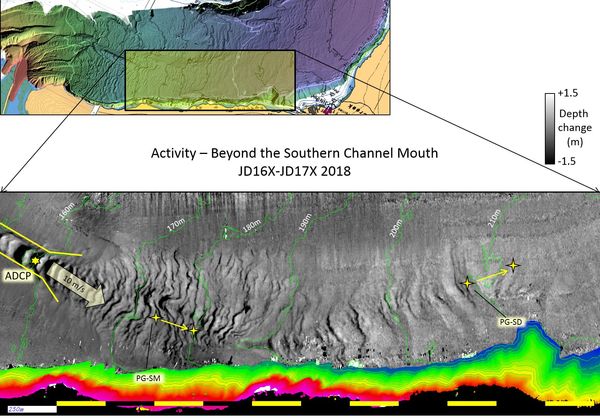
June 15th to June 27th

 |
This was the second ~ 2 week period when
the ADCP was present and when the single strongest flow
event occurred. (The ADCP was monitoring the flow at
all times). As can be seen, the greatest penetration of
the flow occurred in this period, extending almost all the
way to Woodfibre.
What is particularly notable is that the seabed change
beyond the southern channel mouth can be described over
two scales:
- a broad swath affecting the longer wavelength
bedforms,
- within that broad swath, a narrower corridor in
which shorter wavelength bedforms are migrating.
Thus perhaps suggests a higher velocity thinner, perhaps
partially-channelized, flow within a broader, thicker
flow (see explanation figure below). |
June 27th to October
16th
|
This is the last observation period
covering ~ 3.5 months.
The first 3 months of this period, the river discharge
was low (there were no surge events until the
fall). On the 22nd and 28th(?) of September
however, two massive surges occurred. These are probably
responsible for the distal extent of the observable
change.
Note that, the distal change is restricted to a narrower
corridor than the previous epoch. This is the region
with the new shorter wavelength bedforms. This suggests
that the flow this time was thinner than the previous
event. The following figure tries to explain what I
think might.. be happening.
|
Also note that there appear to be two (or three) plausible
pathways downstream of the current southern channel mouth. :
- 1 - directly in line with the channel (this was the
original flow direction and what appears to "ricochet" off
the fjord wall).
- 2- - a new preferred channel that results from flow
capture around a scour pit that developed several years ago.
- 3 - a weak path to the south (upper on these rotated
figures).
The scour pit is an interesting phenomena that has appeared over
the past few years. It is a point of localized scour (around a
pre-existing positive feature of unknown origin) and a train of
bedforms had grown downstream of it, evolving into a headless
channel. It seem to gradually be capturing flow at the expense
of the other two pathways.
Delta
Top Evolution
With the 5 available survey windows, the seasonal evolution of the
delta top channel could be assessed (starting with the over-winter
2017-2018 changes):
Inter-Survey Changes
Improved
delta-top bedform imaging:
All surveys usually utilize the EM710 on board the CSL Heron. This
sonar (70-100 kHz) is designed for ~20-1000m depths and thus is
optimal for the deeper fjords. It is not, however, optimal for the
shallow delta-top river channel. Nevertheless, as it was all we had,
we have always used it (including most notably Danar Pratomo's PhD
thesis).
In 2018, however, we were fortunate to be able to borrow an EM2040P
(200-400 kHz) and used it simultaneously to image the delta top in
late June. The improvement in resolution is illustrated below:
Note that, when reduced to a 1m grid, there is little apparent
difference in morphological definition. At such short ranges,
however, the ability to resolve decimetre wavelength bedforms is of
value.
Locations
of Moorings:
At part of the 2018 program, two hydrophones, 4 pressure gauges and
an ADCP were installed for various period throughout the summer.
This shows the locations of the two
hydrophones (HYPH-North and HYPH-South)
and the four pressure gauges (PG-Cen PG-Nor, PG-Mouth,
PG-Distal).
This shows those same locations over
the cumulative seabed change for the 7month monitoring period in
2018.
As can be seen the two hydrophones are deliberately located between
the three channels on highs that are NEVER affected by flows. Thus
they should hear flows without being dragged. The south
hydrophone should pick up the Southern Channel best, wheres the
north hydrophone should be most sensitive to either Northern or
Central channels. If a flow is heard in both, it gives us an
idea of the range over which we are listening. Also they should not
be in the vertical path of release of bubbles (a point that is
important when trying to understand what it is we are hearing).
For the Pressure gauges, there are two at the proximal end of the
change corridor coming from the Central and Northern channels
respectively.
This is in the hope that we will identify outgoing events
(but not have the gauge destroyed - as was the case in 2017 when we
put one in the Southern Channel just below the constriction).
And for the Southern Channel ,the two pressure gauges are located
well downstream of the mouth of the channel on the unconstrained
lobe. They are deliberately located in the path of the suspected
flows based on inter-survey bathymetric change. The "north" location
is identical to the position of the 2017 mooring. The distal
one is as far out as we suspect any activity at all.
Specific deployed locations are:
- 49 40.7115 -- -123 -11.4797 (49.678525 -123.191328)
Hydrophone_N-C 101m
- 49 40.4019 -- -123 -11.4581 (49.673364 -123.190968)
Hydrophone_C-S 115m
- 49 40.6856 -- -123 -12.1981 (49.678093 -123.203302)
Distal_North 151m
- 49 40.5377 -- -123 -11.8456 (49.675629 -123.197426)
Distal_Central 135m
- 49 40.3742 -- -123 -12.9239 (49.672904 -123.215399)
Mouth_Southern 173m
- 49 39.8897 -- -123 -14.0392 (49.664828 -123.233986)
Distal_Southern 208m
The hydrophones never moved are were replaced either once
(northern) or twice (southern).
The pressure gauges were monitored and located using the EM710 water
column imagery during each on-location survey period. For the whole
period, the Northern and Central Channel moorings appeared to be
almost... in the same place. The other two originally appeared
"lost" after mid June as we we initially were only searching
close to the deployed location.
As it turns out, in the October window they were relocated displaced
~200m downstream, suggesting they had been dragged. Going back
through the survey data, we were then able to monitor when exactly
they moved.
Most interestingly, both of the two most distal pressure gauges
appears to have been dragged that distance, suggesting that the
flows there have significant strength even though this is at the
last trace of seabed change (see later discussion).
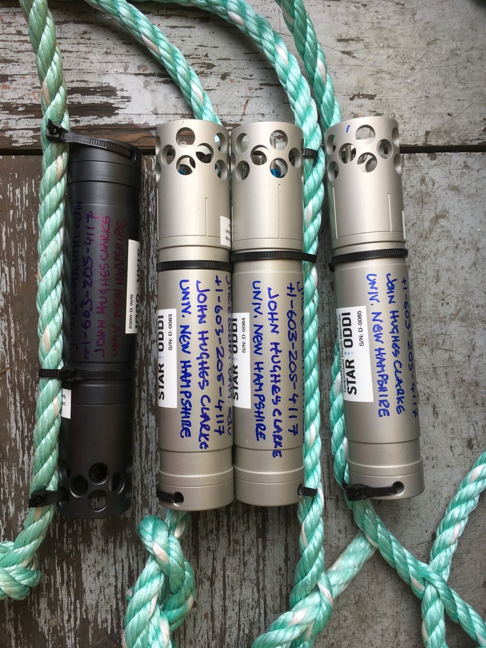
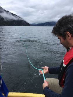
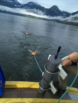
Pressure
Gauge Moorings
Based on the 2017 first testing, pressure gauges, suspended slightly
positively buoyant from mooring blocks are an effective (and
cheap) way of providing long term monitoring of the timing of flows
(see concept in figure below). The instruments used (Starmon_TD
gauges) are capable of logging pressure and temperature at ~
10 second intervals for a period of over a year.

|
still and animation of
PG mooring in EM710 water column
|
the method of detecting
flows using a weakly buoyant pressure gauge
|
showing the unique appearance
of the 5 floats on the mooring
when imaged using the EM710 water column.
(Note the presence of interference rings)
|
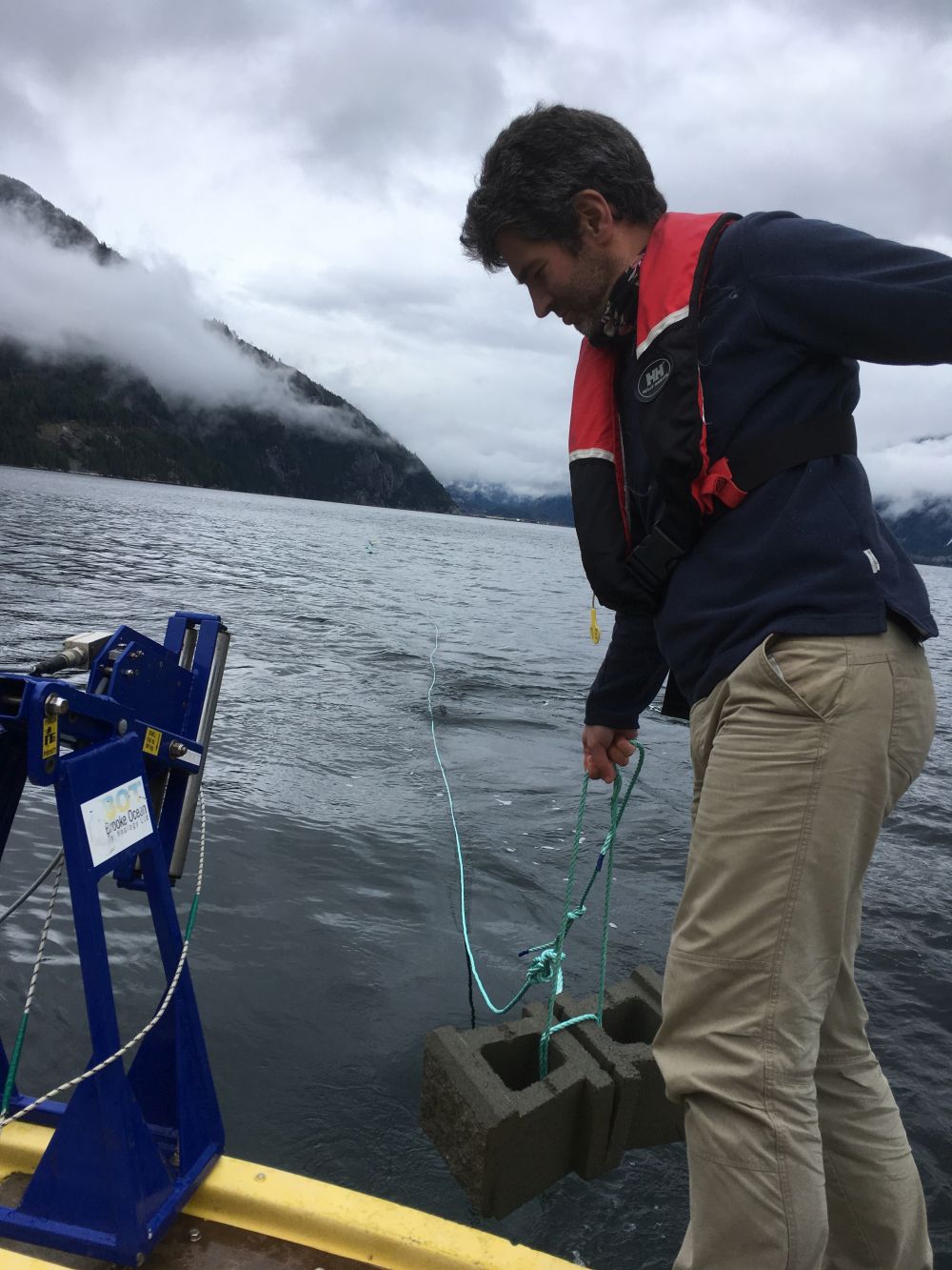
To save on cost, there is no acoustic release (+USD5k). Thus to
recover them requires relocating them and then hooking them with a
grapple array (a clumsy, time-consuming, but feasible
process). The relocation utilizes the thesis algorithm of Carlos
Marques that employs a matched filter to pick out the unique
signature of the vertical line of echo targets in the EM710 water
column imagery (see animation above). Most significantly, for this
year's results, this can identify whether the mooring has been
horizontally dragged without having to recover it.
In 2017, the proximal one in the Southern Channel was ripped out
within the first return period. A lesson not to put these too
proximal. But the distal one, beyond the mouth of the Southern
Channel survived from June to October and was recovered then. It
turned out that the capacitor in it resulted in it stopping after
one month, but it clearly recorded two flows.
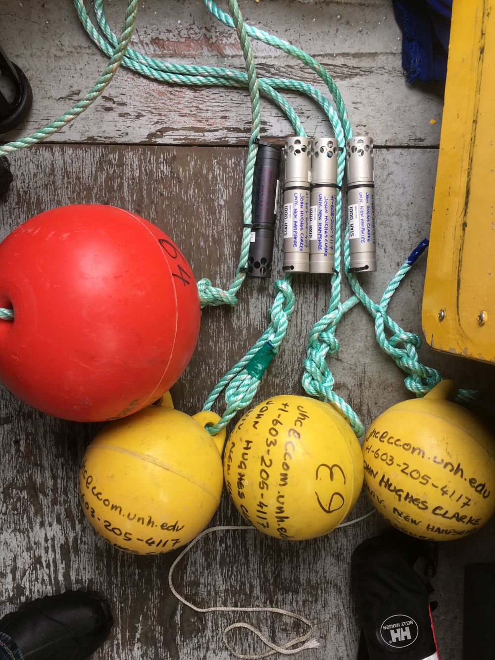
Following on from the 2017 experience in which two pressure
gauges were deployed, this time 4 gauges were deployed. The
logistics of deploying them were identical to 2017:

|

|
|

|
The Starmon-TD sensors
one per mooring
|
mounted just below the highest
float
|
deploying the 4 suspended
buoys
(sensor just above uppermost one)
|
deploying the mooring blocks
(~ 100 lbs)
|
In 2018, 4 locations were selected (see map above):
- the same location beyond the mouth of the south channel.
- a location even more distal beyond the mouth of the south
channel.
- a location directly in the path of the central channel
corridor, but as distal as possible (just before it crosses into
the Southern Channel)
- a location directly in the path of the north channel, but
again just beyond the distal limit of observable bedform
migration
At this time, the location of the 4 gauges has been examined
periodically (whenever a distal survey was run) and their location
measured using the water column imaging method. The sensors seaward
of the Central and Northern channel did not move at all from April
to October. The two distal ones, whose location was estimated during
every on-site survey day, only moved once. In the intervening
period from 15th to 27th of June, when the singular extreme flow
event occurred (10 m/s), both were clearly dragged over 200m
downstream (see figure for details).
 showing the before and after locations of the two distal
pressure gauges
showing the before and after locations of the two distal
pressure gauges
after they had been dragged by the 10m/s event.
Locations superimposed over DTM difference map for the
June 15-27th period.
Recovered Depth/Temperature Signals
As all the pressure gauges have battery life for ~ 18 months, no
attempt was made to recover them during the mid season. In October,
however, it was intended that they would all be recovered,
downloaded and redeployed. In October however, due to the
winch failure, only the pressure gauge at the mouth of the Northern
Channel has been recovered. It did however, log for the full 7
month period (JD097 to JD287) and described a number of interesting
events.
Northern Channel pressure gauge data:

|

|
|
temperature for
the full 7 months
suggesting intrusion in mid September.
|
pressure depth for the
full 7 months
note dominant clear tidal signature
|
depth anomalies
(high-pass filtered < 1 hour) depths
|
|
To put these time series in context, the river discharge for
the same period is shown.
As can be seen, the 4 pressure events occured in August and
early September when the river was weak and declining.
In contrast the three thermal events occurred in late
September when there were river surges.
|
Temperature record:
Although it wasn't envisaged that the data would be terribly useful,
the sensor does automatically log temperature. As it turned out, two
interesting phenomena were noted.
Long Period
Thermal Intrusions:
Unrelated to turbidity current activity, but of interest for local
oceanography, the temperature record indicates that the deep waters
were extremely stable for the first 6 months (cooling slightly), but
that in September the deep waters warmed up slowly over a month (by
~ 0.2 degC) suggesting that warmer Georgia Basin waters had leaked
over the sill downstream. This is of significance for those
modelling the deep flushing of the basin.
Short Period
Thermal Anomalies:
The second thermal anomaly of interest is the series of rapid
temperature spikes that occurred in late September. The figures
below zoom in on the period of interest. Over a period of a few
hours, the deep temperature rose by ~ 0.5 degC and then fell again.
This would suggest that something warm had been injected below the
level of the gauge, and that that warm (less dense) water rose up
through the gauge location.
River Surges in late September
|
Closeup of the first River Surge
|
|
discharge m3/s
|
|
As can be seen, there were two major river
surges at the end of the summer. |
thermal signature during the two river pulses.
|
associated thermal anomalies.
|
Looking at the thermal record, there are
three clear bursts of heat (well +0.4 degC) that appear
closely related to the first river surge.
If one zooms in on the first event, one can see that the
first heat pulse was close to the peak of the river
discharge. The second pulse was on the waning side of the
surge ~ 24 hours later, and the third was 4 days later.
|
|
associated pressure/depth anomalies.
|
As can be seen, there was no depth anomaly so
clearly the pressure gauge was not "tugged" in any way,
associated with these heat pulses.
|
One plausible way that this could happen is that there was a
turbidity current elsewhere (Central or Southern Channels) that
dragged down near-surface warmer water (by September, the river
water is finally hotter than the deep water). That plume spread out,
dropped its excess density due to sediment and gradually rose back
up again.
Notably, the three temperature spikes are associated with the first
of the late September river surges.
If this is really the case, when we get the other three moorings up
they should help us understand what is happening. It will be
interesting to see if they see the same thermal event. And if so,
whether one of the others shows a pressure anomaly indicating that
it was in the path of the associated flow.
Pressure Record:
For the pressure gauge, as expected, the 3-5m range tidal signature
was dominant and extremely clear. This is actually extremely
useful as it allows a means of checking the sensor clock. Ideally it
should match the tide, but by doing the differences (using
correlation) it is apparent that the clock drifted about 10 minutes
over the 7 months. Eventually we will correct the record assuming a
linear drift.
.
Pressure
Anomalies (suggesting events):
Superimposed over the tidal signature at much shorter time scales
(< 1 hour) one would expect that the whole mooring would be
dragged down in the event of a near-seabed flow. This was already
proved from the 2017 data. A 3600 second (1 hr) high pass filter was
used to remove the tide (avoiding the drifting clock problem). This
leaves a slight slowly varying (+/-3cm) tidal signature (related to
the curvature of the tide curve), but nicely reveals any short
period anomalies.
4 significant pressure anomaly events were clear in the whole 7
months - notable all occurred in August and September, long after
the river surges had disappeared. Otherwise the events are very
small (see second row of daily figures), or look like a period in
which the mooring oscillated (see lower two rows).
Future work will be focused on taking out the clock drift so that we
can establish longer period depressions of the mooring (was it
pulled down by burying the rope?). And when the other three are
recovered, see if these events match up between hydrophones,
suggesting propagating flows (or soliton packets).
Hydrophone
Moorings
Based on the experience of Matt Hatcher in 2013, when he had a
10-250 kHz hydrophone deployed for a few hours on top of the
suspended M3's while known turbidity currents were passing, it is
clear that there is a discernible noise emanating from the faster
active flows. His instrument, however, only had battery and storage
for ~ 12 hours. To log data for more than a few days is a challenge
in both battery supply and data storage.
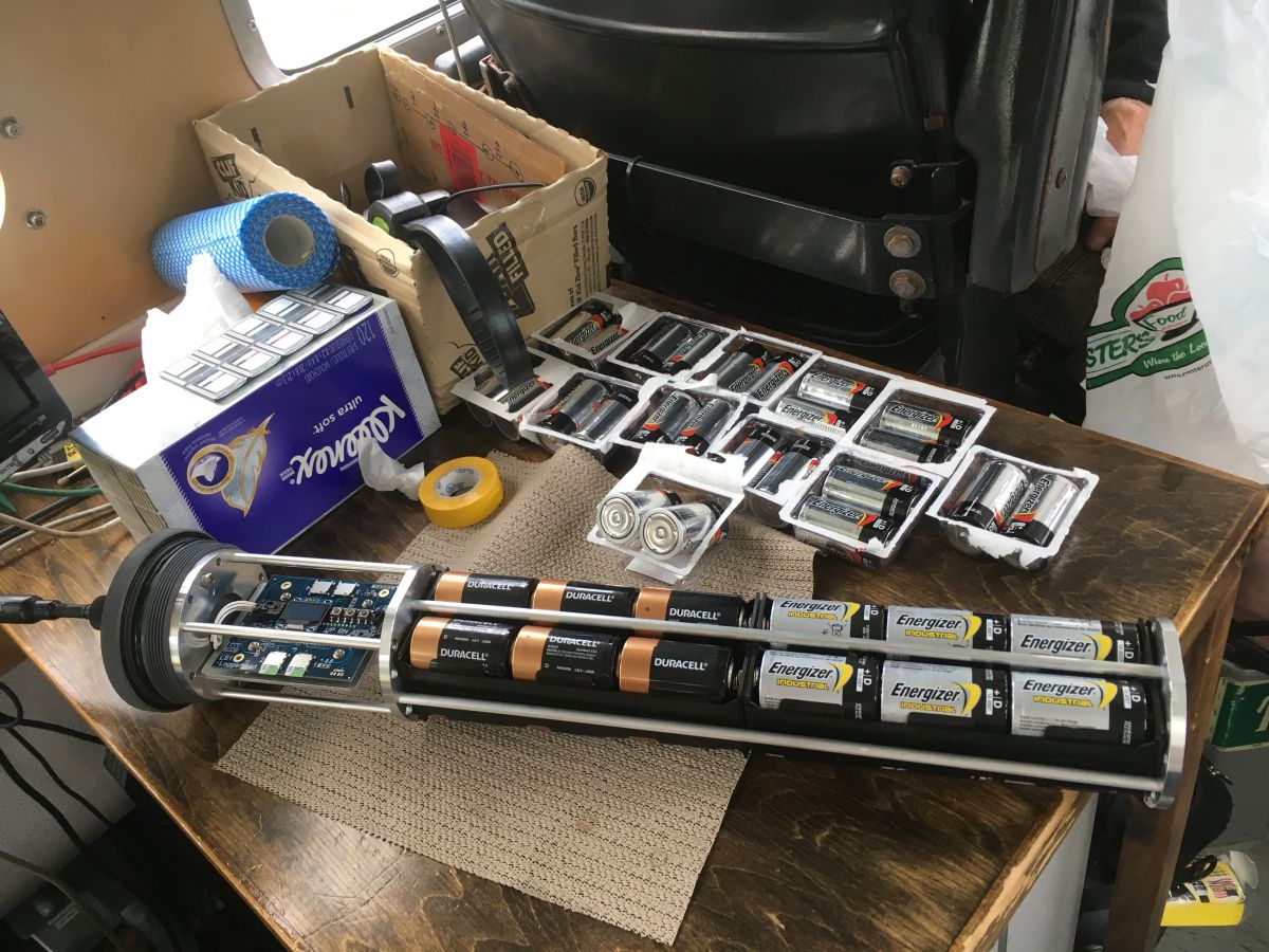
For rapid purchase, affordability and amount of storage and time,
the loggerhead LS1X was chosen. It is capable of logging continuous
data from 1-22 kHz for a period of ~ 2.5 months. They are ~ 24
inches long and were mounted on a mooring that was very visible from
the multibeam water column for the usual grapple recovery.

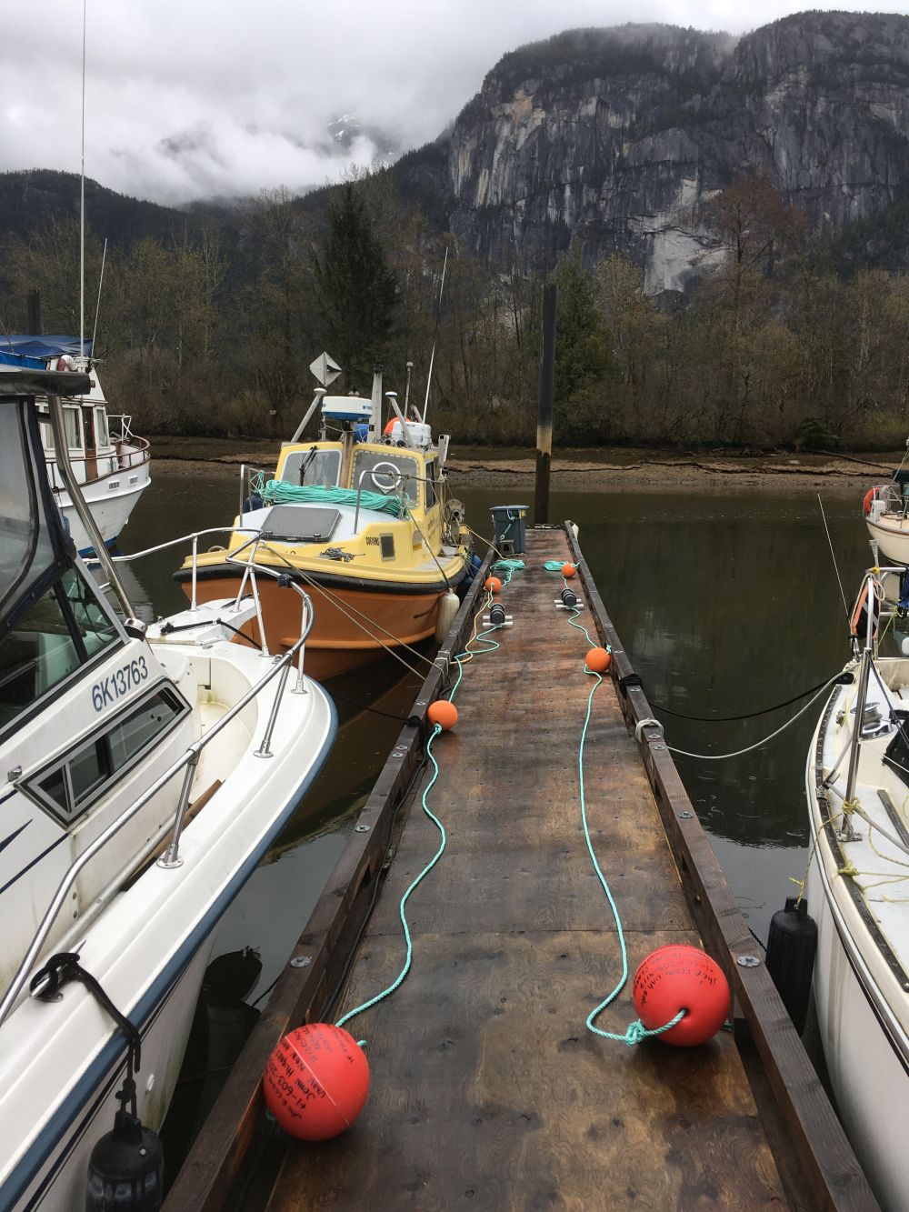
|

|
|
instrument before inserting in
pressure case.
Note 24 D-cells and 4 slots for micro-SD cards.
|
the two moorings as laid out
on
dock before deployment.
|
deploying the mooring -
hydrophone about to go overboard.
|
Raw Data
File (10 minutes) Patterns:
The data consist of consecutive 10 minute wave files recorded at
44.1 kHz. For each 1/4 of a second an FFT is performed on a
tapered window to look at the spectra. The plots below (left) show
the evolution of the spectra (from 0 to 22.05 kHz) over that 10
minute interval. Almost all spectra are red in the sense that there
is more power at lower frequencies. A passing vessel is usually the
loudest noise source and will slowly increase and decrease in
intensity as it passes by. A number of smaller engines produce very
distinct harmonics (specific sets of frequencies). These appear as
stripes in the spectra. They will move as the vessel comes towards
or away from the hydrophone due to the Doppler effect.
Despite all this noise, the signal of interest from the turbidity
currents appear to be characterized by transients. That is to day
the noise is not quasi-continuous, rather it consists of a series of
events ("clicks or clacks") that turn on and off over a matter of a
few seconds (last example shown). These transients can be
distinguished even in the presence of high anthropogenic machinery
noise.
Daily Patterns:
If 144 of these 10 minute files are combined, a 24 hour period may
be examined. It is notable that it is quietest at night reflecting
the dominance of man-made noise. It is also apparent that the port
often prefers their vessels to arrive and depart at night (whether
for reasons of tide or disruption to other traffic is not
clear).
As will be shown in later figures ,the characteristic 15 kHz hiss of
rainfall is quiet distinct (higher than most anthropogenic sounds)
and thus rainfall events can be clearly seen.
Weekly Patterns:
If one collates 7 days one can see if there is any pattern
associated with the working week. As the summer approaches, the
weekend activity of kite-boarders (and especially their supporting
coaches with small outboard motors) can clearly be seen.
As the Heron deliberately steams over the south hydrophone as part
of its repetitive survey activity, her signature can also be clearly
distinguished.
10 Minutes of DATA
|
A DAY of DATA (UTC)
|
A WEEK of DATA
|
all plots:
X axis - 10 minutes
Y axis - 0 -22.1 kHz
colour scale : 50dB dynamic range
two engine sources
broadband (diesel?)
outboard (harmonics)
Heron passing back
and forth overhead.
transients, kiteboarders
and little outboards.
|
the following show spectra for 24 hours:
(144 10 minute files)
(UTC, therefore midnight is 0700)
X axis - 24 hours
Y axis - 0 -22.1 kHz
colour scale : 50dB dynamic range
a rainy night

a noisy night
a quiet night followed by a noisy day.
|
a week of days
(MTWTFSS).
Note
the generally quiet nights.
Sunday night a ship left the port.
|
A typical 24 hour day:
For each day, a 24 hour compilation of the spectra over the day is
generated (example below). Note the 24 hour period is UTC so
midnight is 0700 local time.
one whole day - (April 10th from the Southern
hydrophone).
As can be seen, the night time is the quietest, unless there is a
large ship in the vicinity (the port appears to prefer to schedule
incoming and outgoing vessels overnight, perhaps to avoid civilian
traffic). Otherwise at ~ 0800, it is clear that activity at the
Squamish Terminals (the port) starts and you can here all sorts of
machinery noise. Twice in this particular day, a vessel with
an outboard motor (very specific harmonics) passes by. And a rain
storm starts in the morning. The following examples were all
extracted from the day (April 10th) shown above.
Characteristic Noises:
Heron
Engine/Transmission Noise and KiteBoarder Noise
Another source of noise was the Heron itself and, on windy days and
especially on the weekend, the kite-boarding community. The
two sets of examples below show days when Heron was operating,
specifically around the LLW period when we though that the turbidity
currents might be active in the Southern Channel.
Thursday -- June 14th - 24
hours
Heron running repeated lines over the hydrophone --
blue rectangles
(the racetrack on the Southern Channel)
|
Sunday -- June 17th - 24 hours
Windy weekend - lots of kiteboarders and coach zodiacs
with outboards
(Heron still operating -- blue rectangles)
|
|
 |
|
|
 |
 |
1
minute wave file
can hear outboards stopping and starting and
kitbeboarders moving and falling off.
|
1
minute wave file
can hear outboards stopping and
starting and kitbeboarders moving and falling off. |
|
Identifying Rainfall
To confirm whether the 15 kHz noise is really associated with
rainfall, the meteorological records from Squamish Airport were
compared with the daily spectra. The airport only recorded
cumulative rainfall over a 24 hour period. Nevertheless, from the
figure below, it is clear that those days of accumulation are
clearly those days that the 15 kHz noise shows up.
|
 |
rainfall in the first
deployment.
|
rainfall in the second
deployment
|
Identification of TC associated noise.
To be sure we are really hearing noise associated with a
turbidity current, we have to use data from the one month period
when the ADCP was in place, thus confirming their presence.
What has become apparent is that the stronger flows show up as a
uniquely characteristic series of clicks and clacks (for lack of a
better description). These correspond to rapidly changing spectral
amplitude of time scales of a second or so. To extract such
information, even in the presence of background noise presents a
signal processing challenge. While better approaches may become
apparent later, it was found that simply looking at the high pass
filtered version of the spectrum plot (emphasizing rapid changes in
the spectral intensity) was a reasonably efficient means of
identifying these clicks. To avoid the worst of the anthropogenic
noise, a window centred around 18 kHz was used.

|
 |
showing the daily spectra plot (tides
and river discharge superimposed) when the largest flow
occurred. Within that day, focusing on the 30 minute
period before and during the flow. Note that it was a quiet
night. The first event of the day was an outboard motor, at
~ 1420, followed by the turbidity current at ~ 1440-1450
UTC.
For each 10 minute file, a four frame time series plot is
provided (see below) that shows:
- TOP - Spectral Power (dB) at ~ 18 kHz
- Spectrum over - 0-22 kHz.
- High Pass filtered Spectrum (presented as a
greyscale)
- High Pass filtered Spectral Power at 18 kHz.
|
For the example around this event, two
contrasting noise signatures are highlighted:
LEFT - outboard motor with clear spectral harmonics. Note
that the high pass filtered spectrum shows horizontal lines
(i.e. intensities are fixed in frequency, and continuous in
time.
RIGHT - turbidity current clicks -- in this case the noise
is broad band so vertical stripes - that come and go
abruptly with time.
As the filter is directional, one can separate the vertical
line events from the horizontal line events. Indeed, one can
hear these clicks even in the presences of significant (but
steady) machinery noise.
|
Lets look at the 10 minute files that include the largest flow - the
following plots have the four time series described above:
Not all turbidity currents, however are as loud as the June 24th
even. These show the two 1.5 m/s flows that occurred earlier:
9th June 1.5 m/s event
|
20th June 1.5 m/s event.
|
|
|
The 1.5m/s event on the 9th of
June.
Note how the background is particularly quiet otherwise (no
other noise sources). |
here is a similar flow, but
there is a lot of background (machinery) noise
Even then, however, note that the high pass filter captures
the transient signature and if you listen to the wav file
below you can still here the transients over the machinery. |
|
associated
noise (60 sec. wav file)
|
First Period -
April to end May:
This was a ~ 2 month period, starting well before the freshet, but
including the onset of the first significant flow. Due to logistical
constraints, an ADCP was NOT in place.
The following plots show the timing of the significant transients.
These are periods when there is more than 20 transients in a 1
minute period.
The timing of the transients as heard at the north and south
hydrophone are compared. Times when both appear to be hearing the
same thing are highlighted in bold.
South Channel
Hydrophone:
|
North Channel Hydrophone
|
|
|
Events as indicated by more than 20
transients in a 1 minute period.
|
|
YEAR JD HR MN SC
JD-Day-Month
>20 #
- 2018 127 01 60 50 JD127_07th_05mnth_YES 28
- 2018 132 16 24 35 JD132_12th_05mnth_YES 35
- 2018 132 16 25 35 JD132_12th_05mnth_YES 33
- 2018 132 16 26 35 JD132_12th_05mnth_YES 30
- 2018 132 16 27 35 JD132_12th_05mnth_YES 23
- 2018 132 16 28 35 JD132_12th_05mnth_YES 34
- 2018 132 16 30 35 JD132_12th_05mnth_YES 24
- 2018 132 16 34 37 JD132_12th_05mnth_YES 22
-
- 2018 133 07 37 18 JD133_13th_05mnth_YES 23
- 2018 136 17 14 30 JD136_16th_05mnth_YES 24
- 2018 136 17 16 30 JD136_16th_05mnth_YES 23
- 2018 138 02 39 19 JD138_18th_05mnth_YES 25
- 2018 138 03 03 28 JD138_18th_05mnth_YES 26
- 2018 138 03 23 31 JD138_18th_05mnth_YES 25
- 2018 138 23 19 12 JD138_18th_05mnth_YES 23
- 2018 138 23 21 12 JD138_18th_05mnth_YES 25
- 2018 141 05 08 04 JD141_21th_05mnth_YES 28
- 2018 144 00 17 19 JD144_24th_05mnth_YES 22
- 2018 144 10 17 54 JD144_24th_05mnth_YES 22
- 2018 144 10 18 54 JD144_24th_05mnth_YES 26
- 2018 145 10 48 53 JD145_25th_05mnth_YES 24
- 2018 146 04 39 12 JD146_26th_05mnth_YES 23
- 2018 146 10 09 34 JD146_26th_05mnth_YES 29
- 2018 148 15 03 51 JD148_28th_05mnth_YES 28
- 2018 148 19 23 02 JD148_28th_05mnth_YES 29
- 2018 149 15 53 54 JD149_29th_05mnth_YES 25
|
YEAR JD HR MN SC
JD-Day-Month
>20 #
- 2018 116 00 16 50 JD116_26th_04mnth_YES 71
- 2018 119 19 56 10 JD119_29th_04mnth_YES 59
- 2018 132 16 28 07 JD132_12th_05mnth_YES 25
- 2018 132 16 30 07 JD132_12th_05mnth_YES 24
- 2018 139 20 30 09 JD139_19th_05mnth_YES 24
- 2018 141 05 07 44 JD141_21th_05mnth_YES 21
- 2018 142 19 35 33 JD142_22th_05mnth_YES 27
- 2018 144 10 17 57 JD144_24th_05mnth_YES 22
- 2018 146 04 38 56 JD146_26th_05mnth_YES 26
- 2018 149 15 53 19 JD149_29th_05mnth_YES 37
- 2018 150 17 23 14 JD150_30th_05mnth_YES 27
|
as can be seen, there were 5 notable events that were heard by BOTH
hydrophones.
Second
Period - end May to end May:
This was a ~ 1 month period, in the mid point of the freshet and was
exactly the same duration as the ADCP installation (although the
ADCP memory filled after about 27 days). Thus we can compare the
ADCP recorded flows with the hydrophone detected events (bearing in
mind that the hydrophone is ~1km more proximal than the ADCP on the
southern channel).
The South Hydrophone was recovered at the end of the period, but due
to time constraints (it took ~ 5 hours of grappling to get the South
one), the North Hydrophone was NOT recovered until October (data not
yet analyzed).
Southern Mooring
|
Northern Mooring
|
|
Only recovered in October, Not yet analyzed
|
YEAR JD HR MN
SC JD-Day-Month
>20 #
|
|
Third
Period - end June to whenever the batteries die (July/September?)
At the end of the second period, the south hydrophone was recovered
and the batteries replaced - so it should be good for another 2-3
months. The North hydrophone, however, was not recovered
so was still in place and thus its batteries were expected to run
out within 1-1.5 months. More significantly though, the North
hydrophone had only enough memory for about another 2-3 weeks.
We did in fact recover both of these in October. The South
hydrophone was still powered (LED lit) when we recovered it - but it
ran out of memory on the ~ 19th of September (2.5 months
of logging) - This was, alas, just before the first fall
surge. What is also apparent is that the data were corrupt for
the last 2 weeks of logging though (perhasp due ot low voltage?). No
other analysis has yet been done of either the north or south
hydrophone data as recovered in October.
Fourth
Period - if we were to leave them in over the winter.
We decided to not drop them back in for the Autumn Pineapple
expresses as the winch was broken and it was felt it was safer to
wait until we have acoustic releases in the spring.
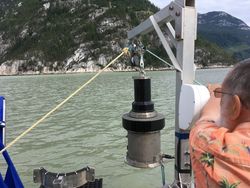
ADCP Mooring
From the 28th of May to the 28th of June, a 600 kHz RDI Sentinel
ADCP was deployed in the usual manner, suspended from a buoy over
the mouth of the South Channel.
3D images - 1-1 (no vertical exaggeration)
showing the ADCP installation
 |
 |
 |
looking upstream
|
close - looking upstream.
|
looking downstream, fjord wall
in the distance.
|
As the period was shorter than usual (4 weeks rather than the max ~6
weeks battery life), a higher ping rate and a shorter ensemble
average period (20 seconds) was used. Within the month, the
batteries survived, but the data disk (only 256 Mb) ran out on the
26th day of a planned 30 day deployment. Nevertheless, based
on the river discharge and surveys from the 26th to the 28th there
were no events in those last two days.
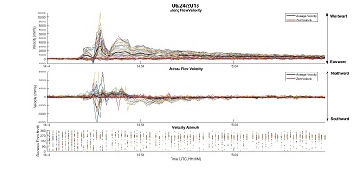
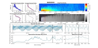
Flows Recorded:
In all, 8 distinct flow events were picked up by the ADCP. Full
details can be found on the page generated by
Liam Cahill.
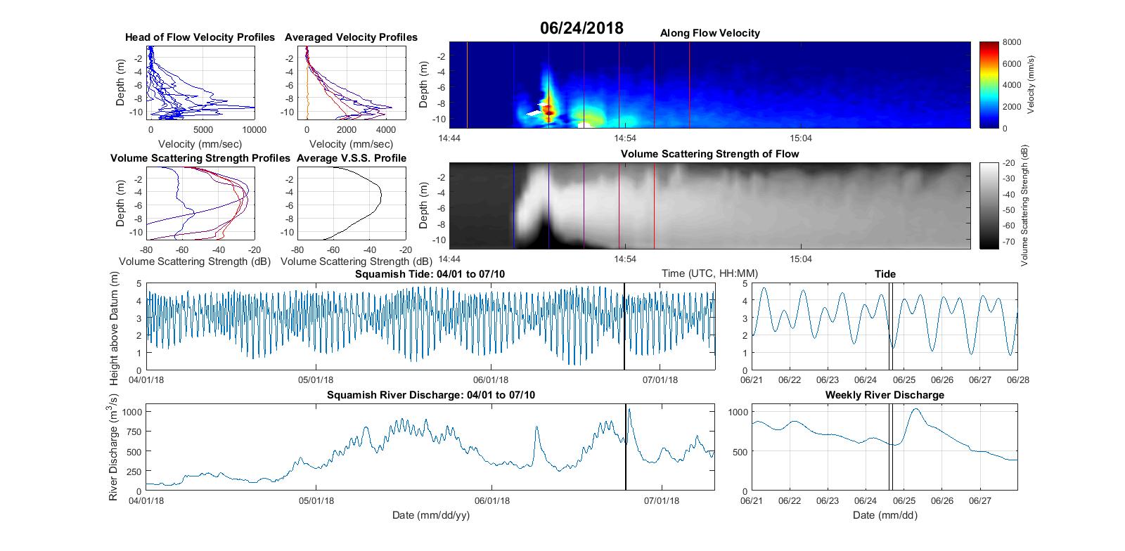
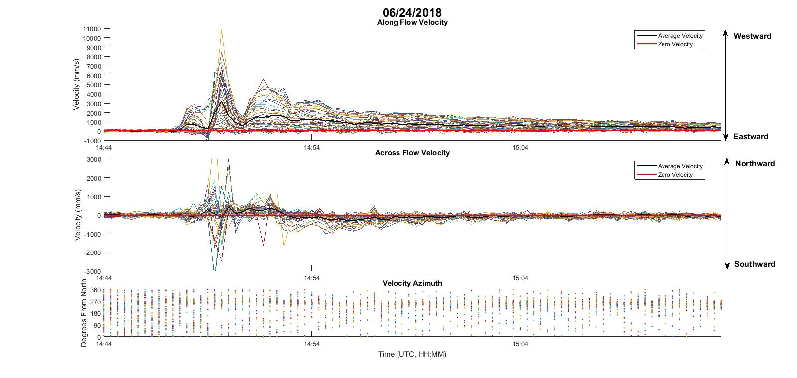
The most powerful event being:
The
10m/s flow
note complete attenuation of
the lower part of the flow
up to 5m off the seabed!
Note also that the 10m/s record only occurred
in a single epoch (20 second averaging).
|
 |
|
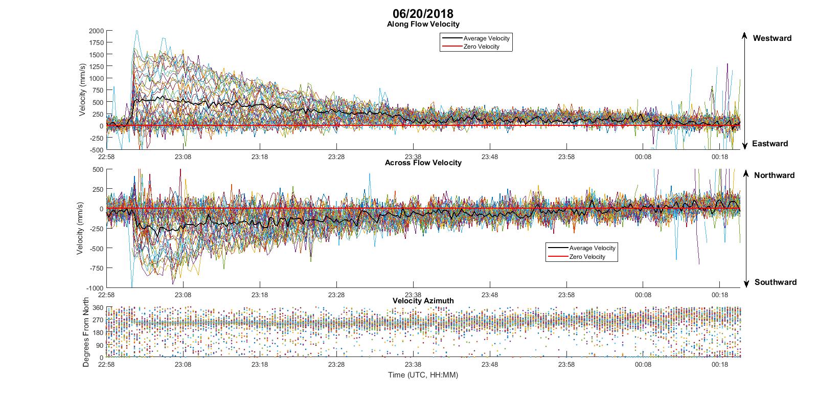
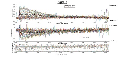
A more typical
1.5m/s flow
note that the base of the
flow is never obscured.
also note that the across channel flow
velocities suggest it may be coming
obliquely from the north channel
(not directly along the south channel).
|
|
|
Timing
of ADCP recorded Events:
Plotted relative to the river discharge and the tidal height.
And plotted relative to the Heron surveys (blue rectangles)
events relative to discharge.
The events are plotted according to their peak velocity
(scale 0-7m/s)
|
same events relative to stage of tide
|
showing Heron survey periods (blue rectangles)
|
showing Heron survey periods (blue rectangles)
|
Comparing
the ADCP event to the South Channel hydrophone mooring upstream:
Over the month period, there were 8 discrete flow events picked up
by the ADCP. Note that the ADCP was at the distal Southern Channel
mouth, whereas the Hydrophone was ~ 1000m upstream. Thus there
would be expected to be more events recorded at the Hydrophone than
at the ADCP (as they could have died out in the intervening period).
The plot below compares the two types of events. As can be seen, of
the 8 flows picked up by the ADCP, only four of them were recognized
by the hydrophone. Notably these were mainly the three FASTEST flows
(1.5, 0.25, 1.5 and > 10.0 m/s). Clearly flows with a speed
of less than 1m/s are not usually discernible (at least using the
current filtering algorithm applied at this point). It is speculated
that the 0.25m/s flow at the ADCP was a lot faster when it passed
the hydrophone, only slowing down downstream.
Additionally, the Hydrophone picked up 11 other events that
qualified (> 20 transients in a minute), none of which correspond
to the ADCP. This could be for one of (or a combination of) two
reasons:
- the flow decelerated after passing the hydrophone and thus did
not make it to the ADCP.
- the transients are caused by another (perhaps man-made)
signature.
This has yet to be further analyzed
|
the top set of lines are the ACDP 8
events
the lines with diamonds are the Hydrophone events
|
The 8 events picked up by the ADCP:
YEAR JD HR MN SC JD-Day-Month_A max m/s
- 2018 160 14 31 13 JD160_09th_Jun_A 1.5
- 16 minutes after
hydrophone
- 2018 165 03 20 53 JD165_14th_Jun_A 0.25
- 45 minutes
after hydrophone.
(perhaps slowing down then?)
- 2018 171 23 01 53 JD171_20th_Jun_A 1.5
- 10 minutes after
hydrophone.
- 2018 172 23 37 53 JD172_21th_Jun_A 0.5
- nothing heard?
- 2018 173 16 51 33 JD173_22th_Jun_A 0.5
- nothing heard?
- 2018 175 14 48 13 JD175_24th_Jun_A 8.0
- during and 6 minutes
after hydrophone
- 2018 176 00 20 53 JD176_25th_Jun_A 0.35
-nothing heard?
- 2018 176 18 48 53 JD176_25th_Jun_B 0.6
-nothing heard?
- -
- ADCP memory filled at ....
in bold are the four that were picked up by the
hydrophone!!!
|
|
|
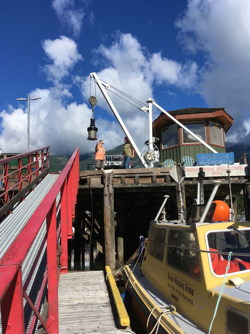
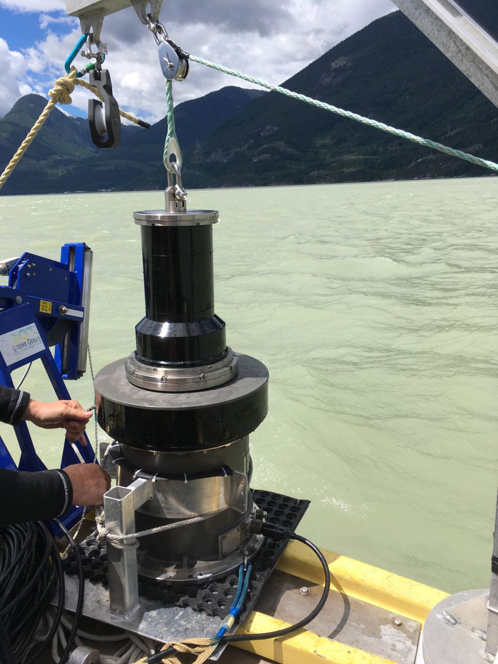
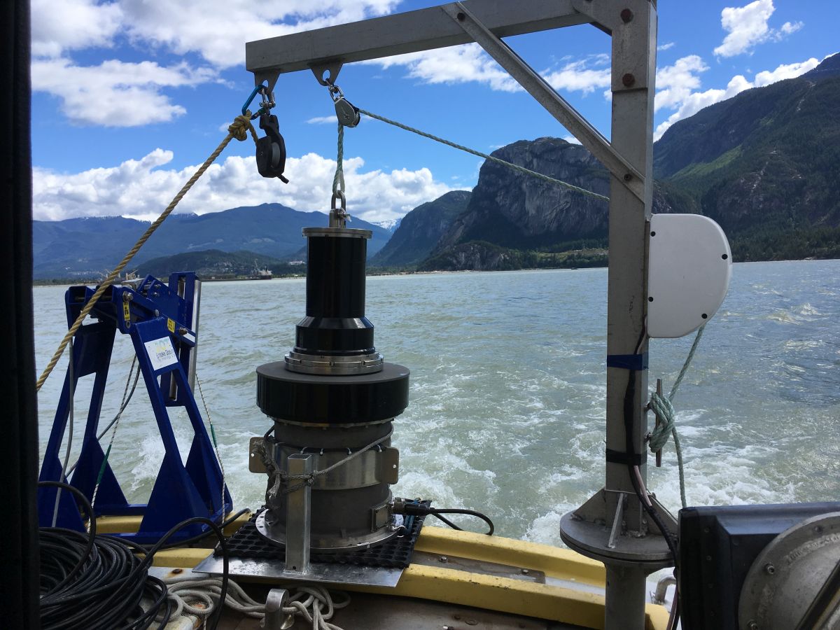
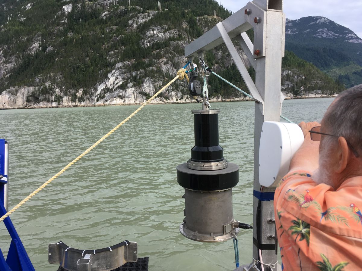
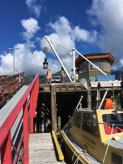
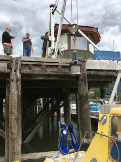
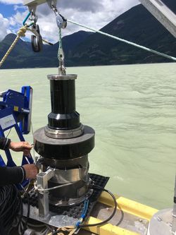
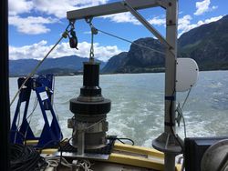
DDS-9001
Imaging
As proposed to Exxon, and with the gratis excellent support of
Konsberg Mesotech (Colin Smith) a DDS-9001-STT was deployed on two
days while drifting at a depth of 48m.
The primary aim this year was to work out the logistics of getting
it there (on and off by pickup) putting it on board (it weights
110kg!), securing it safely and deploying it safely. All this was
achieved with the notable assistance of Mike Boyd who visited
Mesotech for the initial meeting and then designed built and
installed a frame on the transom to take it.
|
|
|
|
|
craning
|
lowering
|
on frame
|
underway
|
being deployed.
|
The following images show the concept
behind the use of the DDS9001 and how it compares to other methods.
The delta lip to ~ 150m contour region of
the prodelta, in which most of the daily activity is
focused.
Traditionally, the method of monitoring activity would be
to bathymetrically resurvey the area periodically. The
whole area would take about 3 hours (and the regions less
than 20m could only realistically be got at high tide).
If only the 3 channel axes are covered, they can be run in
about 1.5 hours. Or a single channel can be run in about
30 minutes (as was done in 2012).
|
showing :
- 1 - the region along the southern channel
axis that was imaged by steaming consecutively along
the channel from a surface vessel (as done in 2017 and
2018).
Each line took about 20 minutes to acquire and thus
that was the update interval.
- 2 - the coverage for the suspended forward looking
M3s (as deployed in 2013). These look at a 120 degree
arc out to a range of 150m. The update rate can be
about half a second if need be.
|
Showing the range achievable using the
DDS-9001. It is a 90 kHz system and has plenty of signal
to noise (with long FM pulses) so can realistically detect
targets (normally divers) out to about that range. The big
issue is the suspended height of the sensor off the
seabed. In this case, owing to cable constraints
(available length) the system was about 40m off the
bottom.
|
Example of a single ping of the DDS-9001
acquired 40m off the bottom at that location.Note the
correspondence of the echo patterns to the topography
(seen in the image to the left).
While the angular resolution decays with range, it
is hoped that an advancing turbidity current (which
suspends massive amounts of gas) would be visible and thus
trackable over a ~ 1600m length of a channel.
Update rate for such imagery is one frame every 2 seconds.
|
2017
CCGS Vector Grab Samples
While not strictly part of the 2018 field operations, over the
summer of 2018 Liam Cahill utilized the Malvern particle size system
belonging to Joel Johnson in Earth Sciences to do the grain size
measurements for the grabs obtained from the CCGS Vector in November
of 2017 (see map below of 19 locations).
location of the 19 grabs acquire by
CCGS Vector in early November, superimposed over a backscatter
mosaic generated by the CSL Heron in late October.
These grabs were located on targets identified from the seabed
backscatter data collected as part of the October 2017 CSL Heron
survey (see figure above). They were designed to see if the clear
patchiness, seen in the EM710 backscatter was any useful indication
of the lithology. The grain sizes are now all done, and the figures
below and in the linked web pages show the results.
 all the grain size - phi units from gravel to clay.
At this time, however, little to no interpretation has been done
(some initial comments are given). What is apparent is that there is
no simple relationship between the backscatter patchiness, as
observed in the EM710 backscatter imagery, and grain size.
What has become apparent (hardly surprising) is that using a grab to
imperfectly recover the top, probably graded, 10-15cm of sediment
(with significant disturbance) is not telling us an awful lot about
the deposit below. The inter-survey differences indicate that a
single event commonly add/removes +/-1m of sediment even in these
distal regions. And we have to be aware that in these low impedance
sediments (high porosity muddy sands) the EM710 at 70-80 kHz is
probably penetrating down partially into that meter.
What is always of interest (at least to me) is that, as with
previous sampling campaigns, there is absolutely nothing lithic out
there coarser than a medium sand, even though the river bedload
includes significant pebble and granule gravel. And also, the
abundant amount of organic debris should not be dismissed. Its
presence may be one of the main controls on the modulation of the
backscatter strength. Even though the organics
themselves are low impedance, associated bubbles (through in-situ
rotting) are probably providing a significant source of scattering.
Ideally a low altitude AUV photographic and high-resolution acoustic
mapping exercise would allow up to look at the thin skinned
sedimentological character of the post-flow sediment--water
interface.
 |
For each grab, we have deck photos and grain
size together with a map of its location relative to the
bathymetry and backscatter as acquired in October 2017
(a week before the grabs were taken).
The following figures provides stills of each one of the
grabs showing grain-size, appearance on deck and location
relative to the bathymetry and backscatter.
The grab coordinates can be found here.
|
South Channel Mouth
Grabs:
A series of grabs were collected in a transect across the
mouth of the South Channel.
What they do clearly demonstrate is that, although the channel
relief is extremely subdued by this point, the flows are clearly
still constrained. Immediately outside the channel,
there is only mud, whereas in the channel floor there is a well
sorted medium sand. This matches the pattern of seabed morphological
change observed at this location.
|

STN29 -- mud (technically poorly sorted fine sand
to coarse silt) to south of channel
|
STN31 -- again, outside the low channel
poorly sorted fine sand with a significant mud
fraction now
|
STN32 -- well sorted medium sand from channel floor -
note that it is not negatively skewed.
|
STN33 -- medium sand with a slight fine tail from just
inside the channel floor.
|
STN34 -- very-fine sand to coarse silt with strong
negative skew from north of the channel
|
Distal Lobe Grabs
6 grabs were collected beyond the distal channel mouth on the
elongate unconstrained corridor that covers the zone in which active
(longer wavelength) bedform migration is seen to occur. There
are notable patchy patterns in the backscatter that appear to
correspond to the lee and stoss faces of these long wavelength
bedforms.
Interestingly though, there is no convincing change in the grain
size distribution associated with the pattern on either side of the
most distal bedforms. They thus may reflect volume scattering from
below the depth to which the grab could reach (> 0.1m). Notably,
the lower backscatter is the more sand rich.
More proximally, all the samples show a well sorted medium sand but
with varying backscatter response. The most notable anomalous
signature appears to come from the presence of significant
organic debris.
For all these samples, there is significant heterogeneity in the
original grab (surface layering probably). As it was moved from the
grab to the container that we received, it was mixed, and then
Liam's choice of subsampling may influence exactly what range of
grainsizes we see.
STN36 -- the higher backscatter in the distal
pattern corresponding to the long wavelength bedforms
two populations - a very fine sand and medium silt.
|
STN37 -- the lower backscatter in the distal pattern
corresponding to the long wavelength bedforms.
poorly sorted very fine sand - pronounced negative skew.
|
STN38 -- in a high backscatter zone in the active
distal corridor. A distinct coarse fraction is present that
reflects unusually high organic matter (crushed leaves
etc..).
fine-very fine sand - the coarse fraction is probably the
organics.
|
STN39 -- in a low backscatter zone in the active
corridor.
Well sorted medium sand.
|
STN40 -- stepping more proximally,
still the reasonably sorted fine sand (now with a fine tail)
but higher backscatter
|
STN41 -- and more proximal again, just down stream of that
growing scour - same higher backscatter, and same well
sorted medium sand,.
|
Distal to
Proximal up the Northern Channel System Channel Floor Grabs
Offset from the dominant Southern Channel system, there is the
possibility of sediment movement coming out of the Northern Channel.
To investigate this, a series of 4 grabs were taken ranging from
distal to proximal (right in the channel).
STN42 -- the most distal, low backscatter zone that is
distinct from the Southern Channel contribution.
very fine sand , pronounced negative skew (fine tail)
|
STN43 -- stepping uphill on the lobe into higher backscatter
fine-very fine sand, quite a fine tail too.
|

STN44 -- just beyond the channelized mouth.
medium-fine sand well sorted - slight fine tail
|
STN45 -- actually in the northern channel floor
medium-fine sand well sorted - slight fine tail
|
Central
Channel floor, levee and more distal
In the past 3-4 years ,the Central Channel had taken over the
Northern Channel as the second most important gateway. The channel
though, ends abruptly and the morphologic change terminates rapidly.
If any sand is moving out onto the lobe, it is likely to spill into
the Southern Channel, thus potentially providing confusion about
where flows that we see at the ADCP site are really coming from.

STN46 -- most proximal grab in the Central Channel axis.
Medium sand with minimal fine tail
|
STN68 -- more distal, but still in the channelized section
of the Central Channel. Still medium and - slightly finer
now with a minor fine trail.
|
STN67 -- this is more distal than the mouth of the Central
Channel.
it was taken to see whether there was any sand coming from
the
Central channel that could be leaking into the Southern
Channel.
Very Fine sands - poorly sorted.
|
STN69 -- this is in the slight high between the Central and
Northern Channels. The idea was to see whether this
constitutes a levee or is experiencing overbank spillage
(the Northern Hydrophone is close to here).
Fine Sand, with a long fine tail.
|
Proximal Southern
Channel
For completeness, a grab was taken in the Southern Channel upstream
of the constriction, to see what is feeding the longest channel in
the system.

STN66 - a well-sorted medium sand.
|
|
Potential
2019 field program
Long term, the aim of continuing the Squamish monitoring program is
to :
- A - extend the monitored period to see long-term morphological
evolution (channel initiation, growth, avulsion etc..)
- B - develop improved technical methods to more completely
understand the full evolution of flow from initiation to deposit
 overview of ideas for improved monitoring
The underlying morphologic monitoring is primarily a seabed mapping
exercise. At a minimum, as long as we can get the Heron there twice
a year, we maintain such a time series. For each year however, the
more we know about the specifics of the event periodicity,
magnitudes and timing, the better we can comprehend why the
morphology is evolving the way it is.
While the 2018 data remain incompletely analyzed, should there be a
continuation of funding the following program is envisaged for the
2019 field season
Spring Startup
- return in April to establish over-winter activity
- do Sandshead channel (Fraser River mouth) in passing.
- recovery of the 3 remaining pressure gauges.
- replace batteries and redeploy all 4 pressure gauges (and
potentially 3 more new ones) for the whole summer.
- buy 3 acoustic releases to facilitate hydrophone recovery.
- deploy the two existing 1-24 kHz - now with acoustic releases.
- purchase an extra hydrophone capable of obtain spectra up to
200 kHz and deploy it too.
June Mission - Hunting for active flows:
- 1 month ADCP deployment
- Within that month, two spring tide windows doing daily
surface survey updates including repetition along southern
channel CLTZ zone.
- rent additional vessel for those two 1-week periods
- from that vessel at a mooring (probably the ADCP site),
suspend DDS-9001 for 6 hours per day (LW +/-3 hours).
- turn over suspended hydrophones to replace batteries and
download data.
August Mission - AUV surveys and groundtruthing.:
- surface survey update
- REMUS - 100 Geoswath AUV surveys of prodelta
region less than 120m (using Brazilian Navy instrument).
- turn over hydrophones (rebattery and download)
October Recovery
- recover hydrophones for winter period
- try recovering and down, loading pressure gauges
- final surveys of year
- do Sandshead system in passing
page developed summer/autumn 2018 by JEHC